import numpy as np
import scipy as sp
import matplotlib.pyplot as plt
def J(x):
return x*np.exp(-x**2) + (x**2)/20
x = np.arange(-10,10,0.1)
y = J(x)
plt.plot(x,y)
plt.xlabel("X")
plt.ylabel("J(X)")
plt.show()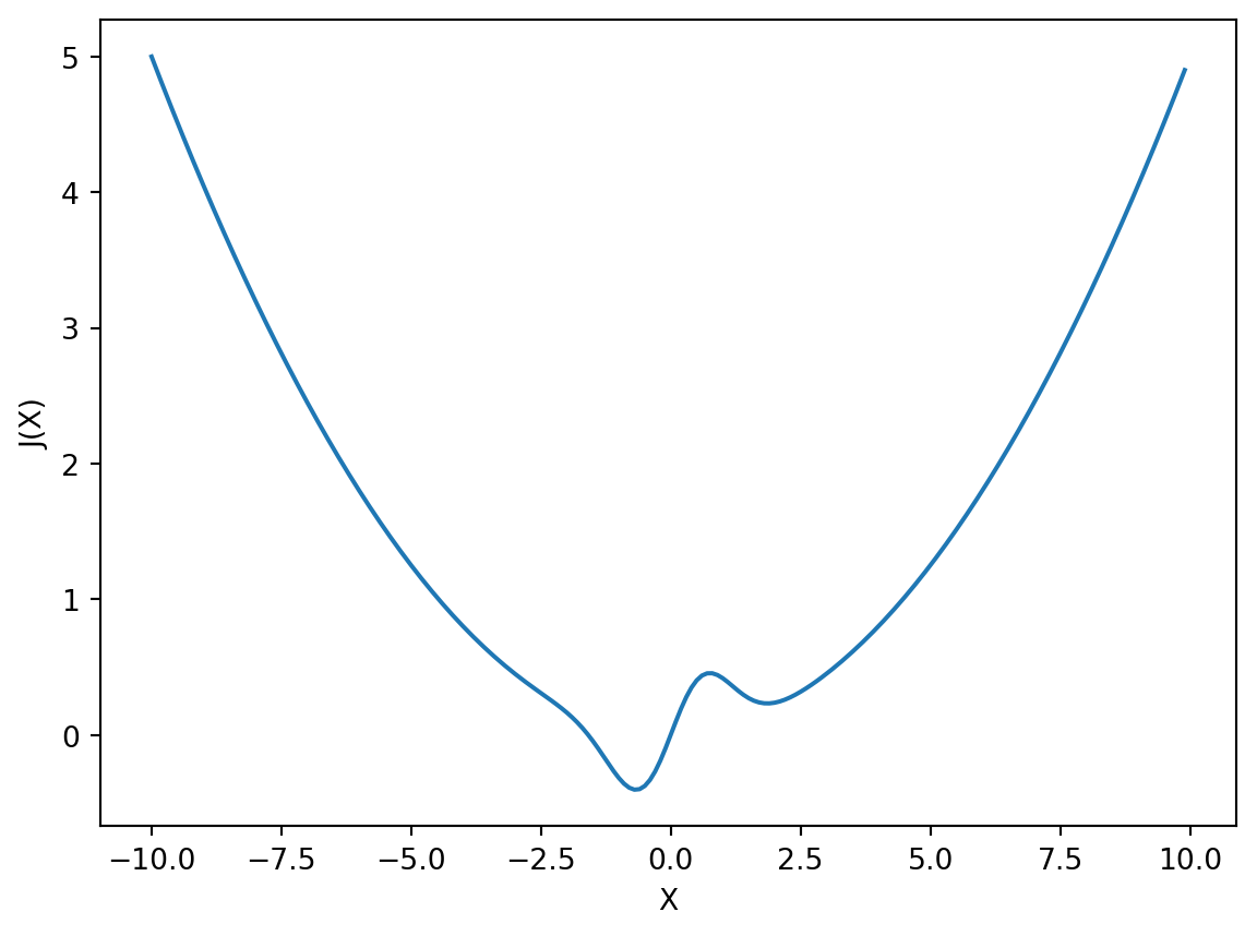
In linear regression, we fit a line of best fit to N samples of (X_{i},Y_{i}) data (i=1 \ldots N) according to a linear equation with two parameters, \beta_{0} and \beta_{1}:
\hat{Y}_{i} = \beta_{0} + \beta_{1} X_{i} + \epsilon_{i}
To find the \beta parameters corresponding to the regression line, we can use a formula that’s based on a procedure called ordinary least squares (OLS). What OLS does is find the \beta parameters that minimize the sum of squared deviations of the estimated values of the data Y (using given values of \beta) and the actual values of Y. That is, the values of \beta_{0} and \beta_{1} that minimize J where:
J = \sum_{i=1}^{N} \left( \hat{Y_{i}} - Y_{i} \right)^{2}
We can call this function J a cost function. The goal then, is to determine, somehow, the values of the parameters \beta_{0} and \beta_{1} that minimize the cost function J.
This is a classic example of an optimization problem. We want to optimize the parameters \beta so that they minimize the cost function J.
Optimization problems abound in science, data analysis, statistical modeling, and even out there in the real world. Here are a few examples, to help you solidify in your mind what optimization is all about, and how it may be used. For some problems (e.g. the shower example) it is easy to think about how you would find the optimal solution. For others, it is not immediately obvious.
Your morning shower: A simple example of optimization is when you hop in the shower and turn on the hot and cold water taps. What you desire is a water temperature that is not too hot, not too cold, but “just right”. The parameters to be optimized are the relative amounts of cold and hot water coming out of the shower head. The cost function is how uncomfortable (whether too cold or too hot) the water temperature is for you.
Tuning a radio: When you tune a radio (an analog radio) and you’re searching for a particular radio station, you are performing an optimization. The parameter you are optimizing is the position of the tuner along the radio spectrum that spans the frequency of the radio station you are trying to listen to. The cost function is the amount of static that you hear overtop of the radio station signal.
Controlling rockets: NASA uses optimization techniques to determine the trajectory of rockets and other spacecraft that will reach their destination using the least amount of fuel. In this case there are parameters that define different trajectories, and a cost function that involves the total amount of fuel burn.
Travelling salesman: A classic example of an optimization problem is the Travelling salesman problem. Given a list of cities and the distances between each pair of cities, what is the shortest possible route that visits each city exactly once and returns to the origin city? In this case the parameters to be optimized are the order of visiting each city, and the cost is the total distance travelled.
Finance: Bankers perform portfolio optimization to determine the mixture of investments that strike the best balance between risk and return. In this case the parameters are the proportions of each type of investment (stocks, bonds, real estate, gold, etc) and the cost function is some (generally secret) equation that balances risk and return.
Statistics: In statistics and data modelling, optimization can be used to find the parameters of a model that best fits the observed data. In this case the parameters to be optimized are the parameters that define the particular model that is being used to model the data (e.g. for linear regression, the \beta values), and the cost function is some measure of goodness-of-fit (actually “badness” of fit). In the case of linear regression, the cost function J is given above.
Machine Learning: Many methods in machine learning, including classification, prediction, etc, are based on optimization: finding the values of model parameters that minimize some cost function. In logistic regression, support vector machines, etc, we find the parameter values that minimize the errors in classifying inputs as belonging to one category vs another (e.g. spam vs non-spam email, or benign vs cancerous tumours, etc). In artificial neural network models, we use optimization to find the values of neuron-to-neuron weights that minimize the network’s errors on an input-output training set.
Neural Network Models: In artificial neural network models, we use optimization to find the values of neuron-to-neuron weights that minimize the network’s errors on an input-output training set. Sometimes the number of parameters to be optimized is very large, even in the millions or billions (e.g. in the case of ChatGPT, ~ 20 billion!)
The Brain?: Some people theorize that some brain functions (e.g. motor control, perception) can be conceptualized as optimization problems. For example for motor cortex, the parameters to be optimized might be the time-varying pattern of action potentials that arrive at \alpha motoneurons in the spinal cord (and hence activate muscles, and move the body) and the cost function might be the amount of beer that is spilled as you move the beer stein from the tabletop to your mouth.
In my lab we have developed MotorNet, an artificial neural network model that learns to control a physiologically realistic mathematical model of an upper arm, according to a cost function that is based on several components including position error, muscle activation, and others. The neural network model learns to control the arm by optimizing the parameters of the neural network model (the weights between neurons) so that the cost function is minimized.
The big question then, is how to determine the parameters that minimize the cost function? There are two general approaches. The analytical approach is to try to find an analytical expression that allows one to directly compute the optimal parameter values. This is wonderful when it can be achieved, because direct calculation is fast. For linear regression using OLS, there exists a matrix equation (shown below) that provides an analytical solution.
For many problems however, it is not possible to find an analytical expression that gives the optimal parameter values. In these cases, one uses a numerical approach to estimate the optimal parameter values (the parameter values that minimize the cost function). As long as you can compute the value of the cost function for a given set of parameter guesses, then you can pursue a numerical approach to optimization. The downside of the numerical approach however is that (1) it can take a long time to converge on the solution, and (2) for some problems, it can be extremely difficult or practically infeasible to converge on the optimal solution.
Optimization is a topic that people can (and have) spent their entire careers studying. It is one of the most important topics in applied mathematics and engineering. We will not attempt to cover the topic in any great breadth. Our goal here is to introduce you to the central idea, and to get some practical experience using numerical approaches to optimization.
In the case of linear regression, there happens to be an analytical expression that allows us to directly calculate the \beta values that minimize J. This is the formula, in matrix format:
\hat{\beta} = \left( X^{\top}X \right)^{-1} X^{\top} Y
In your undergraduate statistics class(es) you may have seen a simpler looking, non-matrix version of this:
\begin{aligned} \hat{\beta_{0}} &= \bar{Y} - \hat{\beta_{1}}\bar{X}\\ \hat{\beta_{1}} &= \frac{\sum\left(Y_{i}-\bar{Y}\right)\left(X_{i}-\bar{X}\right)}{\sum\left(X_{i}-\bar{X}\right)^{2}}\end{aligned}
How do we come up with analytical expressions like these? The answer is Calculus.
It might help to understand the following material by considering a simpler optimization problem, where we have a single paramater \beta to be optimized, for example the position of a radio tuner as you hone in on your favourite radio station. Call the position of the tuner dial \beta. What we want is to find the value of \beta that minimizes the cost function J, where J is, for example, the amount of static that you hear overtop of the radio station signal. Let’s say we’re searching the airwaves for Virgin Radio but you’ve forgotten the frequency (97.5 MHz). We can visualize a hypothetical relationship between \beta and J graphically, as shown in Figure 1.
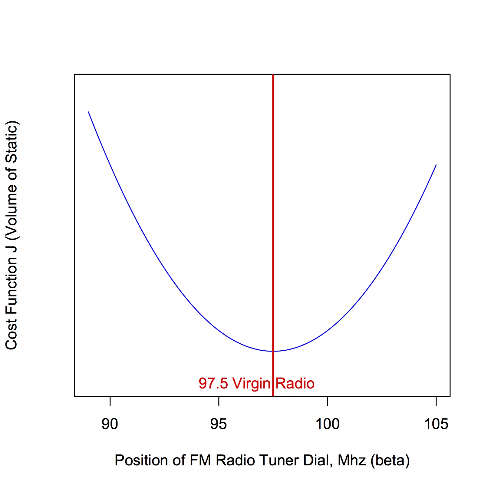
As we move the dial under or over the actual (forgotten) frequency for Virgin Radio, we get static and the cost function J increases. The farther we move the dial away from the 97.5 MHz frequency, the greater the cost function J. What we desire is the frequency (the value of \beta) corresponding to the bottom (minimum) of the cost function, i.e. the minimum value of J.
We can remember from our high school calculus days that at the minimum of a function f, the first derivative of f equals zero. With respect to our Virgin Radio example, this means that the derivative of J with respect to \beta is zero at the minimum of J. In equation form with calculus notation, what we want to derive is an expression that gives us the value of \beta for which the first derivative of \beta with respect to J is zero:
\frac{\partial{J}}{\partial{\beta}} = 0
If we can write an algebraic expression to describe how J varies with \beta, then there’s a chance that we can do the differentiation and arrive at an analytical expression for the minimum. A very simple toy example: let’s say we can write J(\beta) as:
J = 10 + \left(\beta - 97.5\right)^{2}
Now in this little example one doesn’t need calculus to see that the way to minimize J is to set \beta = 97.5. Let’s pretend however that we couldn’t see this solution directly (as is often the case with more complex cost functions—for example for linear regression and OLS). If we take the derivative of J with respect to \beta, we get:
\begin{aligned} \frac{\partial{J}}{\partial{\beta}} &= 0\\ \frac{\partial [ 10 + (\beta-97.5)^{2} ]}{\partial \beta} &= 0\\ 2\left(\beta - 97.5\right) &= 0\\ 2 \beta &= 2 (97.5)\\ \beta &= 97.5\end{aligned}
So in this little example the analytical expression for the optimal value of \beta isn’t even an expression per se, it’s an actual value.
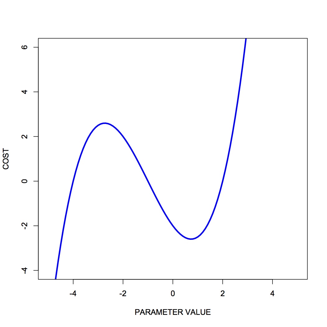
Note also that technically, that the slope of a function is zero not only at a minimum but also at a peak. If we truly want to find only minima then we should also look for places where the second derivative (the slope of the slope) is positive. Parameter values where the first derivative is zero and the second derivative is positive, correspond to valleys. Parameter values where the first derivative is zero and the second derivative is negative, correspond to peaks. Draw a function with a peak and a valley, then draw the first and second derivatives, to convince yourself that this is true. See Figure 2 for an example of a function with a peak and a valley.
For some optimization problems, doing the calculus to find an analytical expression for the optimal parameter values is possible. For many optimization problems however, the calculus simply cannot be done. In this case our only option is to pursue a numerical approach. This is what we will focus on in this course—numerical approaches to optimization.
In numerical approaches to optimization, the general idea is that you pursue an iterative approach in which you guess at optimal parameter values, you evaluate the cost, and then you revise your guess. This loop continues until you decide to stop, for example when continued iterations don’t reduce your cost below some amount you decide is small enough.
Numerical approaches can be distinguished as local versus global methods. Local methods use only local information about the relationship between cost and parameter values in the local “neighborhood” of the current guess. Global methods involve multiple guesses over a broad range of parameter values, and revised parameter guesses take into account information from all guesses across the entire parameter range.
In local numerical approaches to optimization, the basic idea is to:
start with an initial guess at the optimal parameter values
compute the cost at hose parameter values
is the cost low enough? If yes, stop. If no, continue
estimate the local gradient at the current parameter values
take a step to new parameter values using the local gradient info
go to step 2
Sometimes at step 2, the stopping rule looks at not just the current cost but also other values such as the magnitude of the local gradient. For example if the local gradient gets too shallow then the stopping rule might get triggered.
You can think of this all in real-world terms in the following way. Imagine you’re heli-skiing in the back-country, and at the end of the day instead of taking you back to Whistler village, your helicopter pilot drops you somewhere on the side of Whistler Mountain. Only problem is, it’s extremely foggy and you have no idea where you are, or which way is down to the village. You can only see 3 feet in front of you. All you have on you is an altimeter. What do you do? Probably something akin to the iterative numerical approach of gradient descent.
You have to decide which way is downhill, and then ski in that direction. To estimate which way is downhill you could do something like the following: take a step in three directions around a circle, and for each step, check the altimeter and compare the altitude to the altitude at the center of the circle. The step corresponding to the greatest altitude decrease represents the steepest “downhill”.
Then you have to decide how long to ski in that direction. You could even tailor this ski time to the local gradient of the mountain. The steeper the slope, the smaller the ski time. The shallower the slope, the longer the ski time.
When you determine that moving in any direction doesn’t decrease your altitude very much, you conclude that you’re at the bottom.
This is essentially how numerical approaches to optimization work, by doing iterative gradient descent. Think about the ski hill example, and what kinds of things can go wrong with this procedure.
One common challenge with complex optimization problems, is the issue of local minima. In the bowl-shaped example of a cost function that we plotted above, there is a single global minimum to the cost function—one place on the cost landscape where the slope is zero. It happens often however that there are local minima in the cost function—parameter values that correspond to a flat region of the cost function, where local steps will only increase the cost—but for which the cost is not the global minimum cost. Figure 3 shows an example of such a cost function.
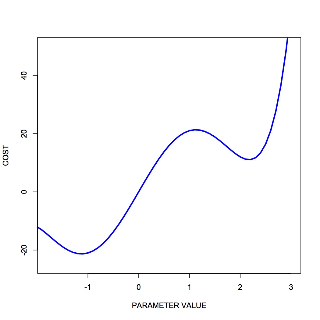
You can see that there is a single global minimum at a parameter value of about -1—but there is a second, local minimum at a parameter value of about 2.2. You can see that if our initial parameter guess was between 1.5 and 3.0, that our local gradient descent procedure would put us at the local minimum, not the global minimum.
One strategy to deal with local minima is to run several gradient descent runs, each starting from a different (often randomly chosen) initial parameter guess, and then to take the best one as the global minimum. Ultimately however in the absence of an analytical solution, or a brute force mapping of the entire cost landscape (which is often infeasible) one can never be sure that one isn’t at a local versus a global minimum.
A number of effective algorithms have been developed for finding parameter values that minimize a cost function. Some don’t assume any pre-existing knowledge of the gradient—that is, of the derivative of the cost function with respect to the parameters, while some assume that we can compute both the cost and the gradient for a given set of parameter values.
In simple gradient descent, the simple idea is as described above, namely to estimate the local gradient and then take a step in the steepest direction. There are all sorts of ways of defining the step size, and adapting the step size to the steepness of the local gradient. There are also terms one can add that implement momentum, as a scheme to try to avoid local minima. Another strategy is to include randomness, by implementing stochastic gradient descent.
In conjugate gradient descent, one requires knowledge of the local gradient, and the idea here is that the algorithm tries to compute a more intelligent guess as to the direction of the cost minimum.
In Newton’s method, one approximates the local gradient using a quadratic function, and then a step is taken towards the minimum of that quadratic function. You can think of this as a slightly more sophisticated version of simple gradient descent, in which one essentially approximates the local gradient as a straight line.
The Nelder-Mead (simplex) method is an iterative approach that is pretty robust, that has an interesting geometric interpretation (see the animation on the wikipedia page) that is not unlike the old toy called Wacky Wally.
There are more complex algorithms such as Levenberg-Marquardt and others, which we won’t get into here.
The bottom line is that there are a range of local methods that vary in their complexity, in their memory requirements, in their iteration speed, and their susceptability to getting stuck in local minima. My approach is to start with the simple ones, and add complexity when needed.
In global optimization, the general idea is instead of making a single guess and descending the local gradient, one instead makes a large number of guesses that broadly span the range of the parameters, and one evaluates the cost for all of them. Then the update step uses the costs of the entire set of guesses to determine a new set of guesses. It’s also an iterative procedure, and when the stopping rule is triggered, one takes the guess from the current set of guesses that has the lowest cost, as the best estimate of the global minimum.
Global methods are well suited to problems that involve many local minima. Going back to our ski hill example, imagine instead of dropping one person on the side of Whistler mountain, rather a platoon of paratroopers is dropped from a plane and scattered all over the entire mountain range. Some will end up in valleys and alpine lakes (local minima) but the chances are good that at least one will end up in whistler village, or close to it. They all radio up to the airplane with their reported altitudes, and on the basis of an analysis of the entire set, a new platoon is dropped, and eventually, someone will end up at the bottom (the global minimum).
Two popular global methods you might come across are simulated annealing and genetic algorithms. Read up on them.
MATLAB has many different functions in the Optimization Toolbox for doing optimization, depending on whether you are doing linear vs nonlinear optimization, whether you have constraints or your problem is unconstrained, and other considerations as well. See the MATLAB documentation for all the details.
Here we will consider unconstrained nonlinear optimization, and later we will look at curve fitting.
There are two main functions to consider in MATLAB for doing unconstrained, nonlinear optimization: fminsearch (which uses Nelder-Mead simplex search) and fminunc (which uses gradients to search).
The MATLAB documentation contains some guidelines about when to use these different functions:
“
fminsearchis generally less efficient thanfminuncfor problems of order greater than two. However, when the problem is highly discontinuous,fminsearchmight be more robust.”
There is also a page in the MATLAB documentation that gives a more comprehensive set of guidelines for when to use different optimization algorithms:
Here is a simple example of a one-dimensional (one parameter) optimization problem. Consider the following function J of a single parameter x:
J(x) = x \mathrm{e}^{(-x^{2})} + \frac{x^{2}}{20}
Assume values of x range between -10.0 and +10.0.
Let’s first generate a plot of the cost function J over the range of x. The code is shown below and the plot is shown in Figure 4.
J = @(x) x.*exp(-x.^2) + (x.^2)/20;
x = -10:0.1:10;
y = J(x);
plot(x,y)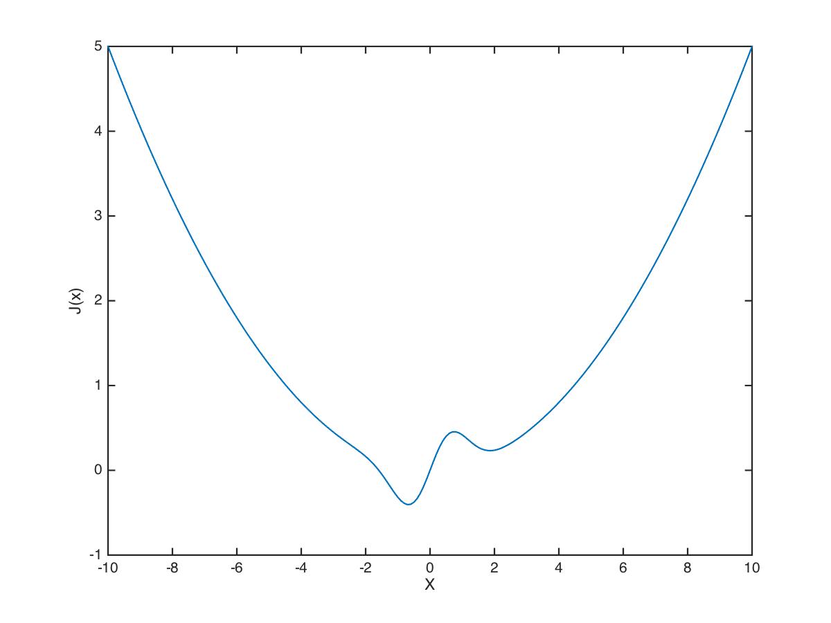
We can see that there is a global minimum between -2.0 and 0.0, and there also appears to be a local minimum between 0.0 and 3.0. Let’s try using the fminsearch function to find the value of x which minimizes J(x):
>> [X,FVAL,EXITFLAG] = fminsearch(J,0.0)

X =

   -0.6691


FVAL =

   -0.4052


EXITFLAG =

     1
We can see that the optimizer found a minimum at x=-0.6691, and that at that value of x, J(x)=-0.4052. It appears that the optimizer successfully found the global minimum and did not get fooled by the local minimum.
Let’s try a two-dimensional problem:
J(x,y) = x \mathrm{e}^{(-x^{2}-y^{2})} + \frac{x^{2}+y^{2}}{20}
Now we have a cost function J in terms of two variables x and y. Our problem is to find the vector (x,y) that minimizes J(x,y).
Let’s write a function file for our cost function:
function J = mycostfun2d(X)
%
% note use of dot notation on .* and ./ operators
% this enables the computation to happen for
% vector values of x
%
x = X(:,1);
y = X(:,2);
J = (x .* exp(-(x.*x)-(y.*y))) + (((x.*x)+(y.*y))./20);
Let’s plot the cost landscape, which is shown in Figure 5:
x = linspace(-3,3,51);    % sample from -3 to +3 in 50 steps
y = linspace(-3,3,51);
XY = combvec(x,y);
J = mycostfun2d(XY');     % compute cost function over all values
[Y,X] = meshgrid(x,y);    % reshape into matrix form
Z = reshape(J,length(x),length(y));
figure                    % visualize the cost landscape
meshc(X,Y,Z);
shading flat
xlabel('X');
ylabel('Y');
zlabel('J');
Now let’s use fminsearch to find the values (x,y) that minimize J(x,y):
>> [Xf,FVAL] = fminsearch('mycostfun2d', [5,5])

Xf =

   -0.6690   -0.0000


FVAL =

   -0.4052
Let’s plot our solution to verify it looks reasonable—this is shown in Figure 6:
hold on
z0 = get(gca,'zlim');
z0 = z0(1);
plot3([Xf(1),Xf(1)],[get(gca,'ylim')],[z0 z0],'color','r','linewidth',2);
plot3([get(gca,'xlim')],[Xf(2),Xf(2)],[z0 z0],'color','r','linewidth',2);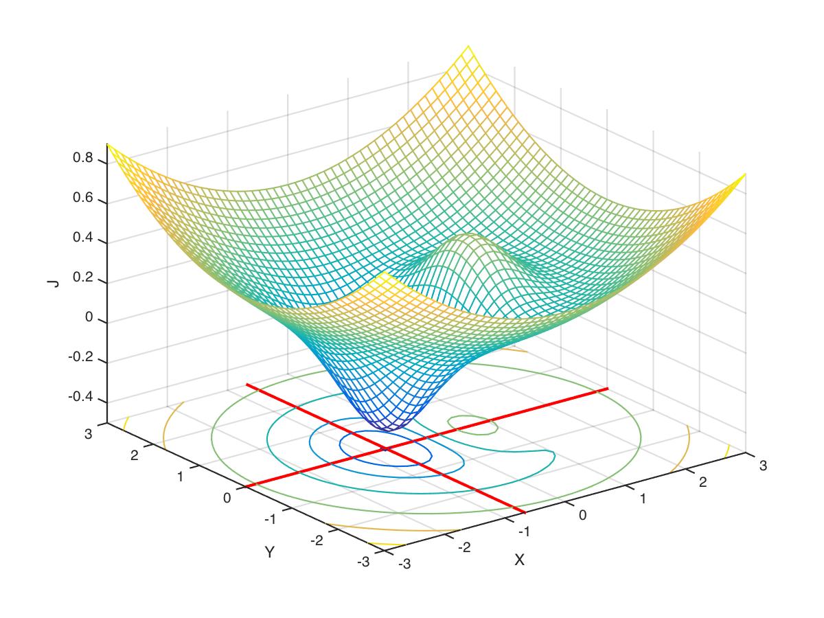
We can do nonlinear least squares curve fitting in MATLAB using lsqcurvefit(). There is also a GUI tool for curve fitting in MATLAB called cftool().
In Python the SciPy package includes many functions for optimization. The SciPy documentation contains a good overview of the different optimization algorithms available in SciPy: scipy.optimize.
The scipy.optimize.minimize() function is a general-purpose function for the minimization of a scalar function of one or more variables. It can use many different gradient descent algorithms including Nelder-Mead, congujate gradient descent, and others. The SciPy documentation for minimize() is here.
Let’s repeat the example from the MATLAB section above, but this time using Python and SciPy. First we define the cost function:
J(x) = x \mathrm{e}^{(-x^{2})} + \frac{x^{2}}{20}
Assume values of x range between -10.0 and +10.0.
Let’s first generate a plot of the cost function J over the range of x.
import numpy as np
import scipy as sp
import matplotlib.pyplot as plt

def J(x):
    return x*np.exp(-x**2) + (x**2)/20

x = np.arange(-10,10,0.1)
y = J(x)
plt.plot(x,y)
plt.xlabel("X")
plt.ylabel("J(X)")
plt.show()
Now let’s use the minimize() function to find the value of x that minimizes J(x):
opt_out = sp.optimize.minimize(J,0.0)
print(opt_out)
print(f"\nthe value of x that minimizes J(x) is {opt_out.x[0]:.4f}")
print(f"the value of J(x) at {opt_out.x[0]:.4f} is {opt_out.fun:.4f}")
message: Optimization terminated successfully.
success: True
status: 0
fun: -0.4052368702666855
x: [-6.691e-01]
nit: 5
jac: [-1.192e-07]
hess_inv: [[ 5.251e-01]]
nfev: 12
njev: 6
the value of x that minimizes J(x) is -0.6691
the value of J(x) at -0.6691 is -0.4052J(x,y) = x \mathrm{e}^{(-x^{2}-y^{2})} + \frac{x^{2}+y^{2}}{20}
Now we have a cost function J in terms of two variables x and y. Our problem is to find the vector (x,y) that minimizes J(x,y).
Let’s write a function file for our cost function:
def J(X):
    x = X[0]
    y = X[1]
    return x*np.exp(-(x**2)-(y**2)) + ((x**2)+(y**2))/20
Let’s plot the cost landscape:
from matplotlib import cm
x = np.arange(-3,3,0.1)
y = np.arange(-3,3,0.1)
XY = np.array(np.meshgrid(x,y)).T.reshape(-1,2) # create a grid of x,y values
Z = np.array([J(xy) for xy in XY]) # compute cost function over all values
Y,X = np.meshgrid(x,y) # reshape into matrix form
Z = Z.reshape(X.shape) # reshape into matrix form
fig, ax = plt.subplots(subplot_kw={"projection": "3d"})
surf = ax.plot_surface(X,Y,Z, cmap=cm.coolwarm, linewidth=0, antialiased=False)
ax.set_xlabel("X")
ax.set_ylabel("Y")
ax.set_zlabel("Z")
Text(0.5, 0, 'Z')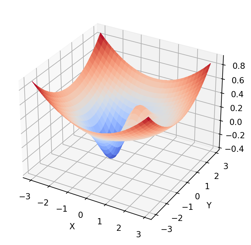
Now let’s use sp.optimize.minimize() to find the values (x,y) that minimize J(x,y):
opt_out = sp.optimize.minimize(J,[5,5])
print(opt_out)
print(f"\nthe value of (x,y) that minimizes J(x) is ({opt_out.x[0]:.4f},{opt_out.x[1]:.4f})")
print(f"the value of J(x) at ({opt_out.x[0]:.4f},{opt_out.x[1]:.4f}) is {opt_out.fun:.4f}")
message: Optimization terminated successfully.
success: True
status: 0
fun: -0.4052368702645366
x: [-6.691e-01 7.061e-07]
nit: 9
jac: [-2.682e-06 6.855e-07]
hess_inv: [[ 5.387e-01 -6.259e-03]
[-6.259e-03 1.050e+00]]
nfev: 48
njev: 16
the value of (x,y) that minimizes J(x) is (-0.6691,0.0000)
the value of J(x) at (-0.6691,0.0000) is -0.4052A common use of optimization is fitting a mathematical function to a set of (usually noisy) data.
Let’s generate some noisy data:
np.random.seed(2023)
x = np.linspace(0, 7, 100)
y = 5 + 3*x + 1*(x-4)**2 + np.random.randn(len(x))
plt.plot(x,y,'bo')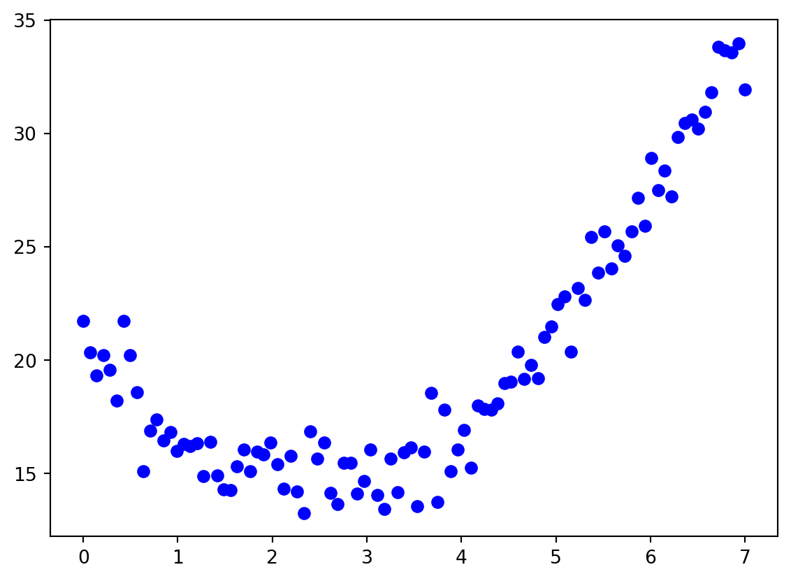
Now let’s say we want to fit a function of the following form to the data:
y = \beta_{0} + \beta_{1}x + \beta_{2}(x+\beta_{3})^{2}
The function has four parameters \beta_{0}, \beta_{1}, \beta_{2}, and \beta_{3}.
Let’s write a Python function that computes the value of the function for a given set of parameters, and the x and x data:
def myfun(beta,x,y):
    return beta[0] + beta[1]*x + beta[2]*(beta[3]+x)**2
Let’s say we want to fit the function using ordinary least squares, in other words we want to find the four parameters that minimize the sum of squared differences between the function and the data.
Now we can feed myfun() any guess at the four \beta values and it will return y:
yhat = myfun([2,3,4,-5],x,y)
plt.plot(x,y,'bo')
plt.plot(x,yhat,'r--')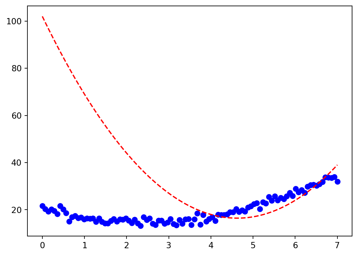
We can see the fit is poor! Now we can use an optimizer to find the four \beta values that minimize the sum of squared differences between the function and the data. Let’s first define our cost function that computes the sum of squared differences between the function and the data:
def mycost(beta,x,y):
    return np.sum((myfun(beta,x,y) - y)**2)
Now we can use minimize() to find the values of \beta that minimize the cost function:
opt_out = sp.optimize.minimize(mycost,[2,3,4,-5],args=(x,y))
print(opt_out)
beta_opt = opt_out.x
yhat = myfun(beta_opt,x,y)
plt.plot(x,y,'bo')
plt.plot(x,yhat,'r-',linewidth=2)
message: Optimization terminated successfully.
success: True
status: 0
fun: 124.2188945215292
x: [-7.022e+00 5.602e+00 9.856e-01 -5.295e+00]
nit: 15
jac: [ 2.861e-06 6.676e-06 7.629e-06 7.629e-06]
hess_inv: [[ 1.933e-01 -3.532e-02 -7.497e-03 1.603e-03]
[-3.532e-02 6.774e-03 1.351e-03 -2.672e-04]
[-7.497e-03 1.351e-03 3.644e-04 -2.162e-05]
[ 1.603e-03 -2.672e-04 -2.162e-05 4.491e-05]]
nfev: 100
njev: 20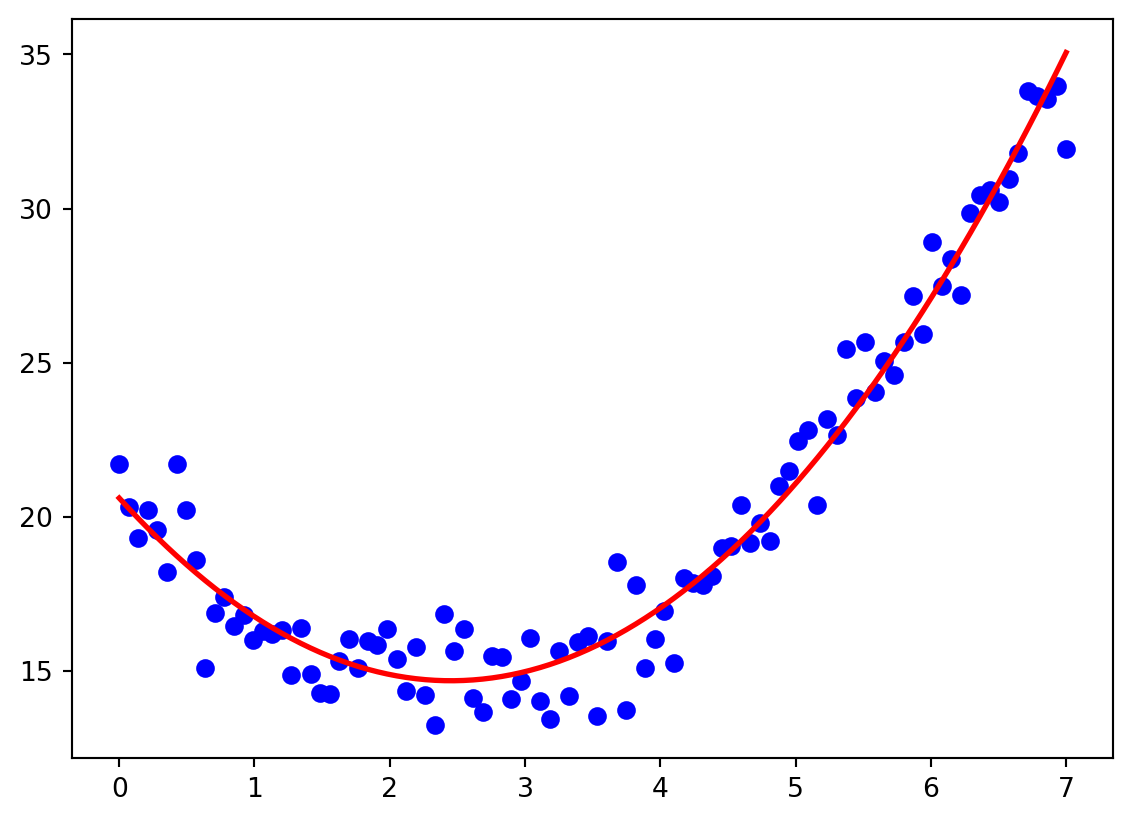
Notice how in the function call to sp.optimize.minimize() we pass an argument args=(x,y) that contains the x and y data. This is how we pass additional arguments (arguments in addition to the array of beta parameters) to the cost function.