# our dependent variable: memory score
memoryscore <- c(7.0, 7.7, 5.4, 10.0, 11.7, 11.0, 9.4, 14.8, 17.5, 16.3)

# a Factor coding the group membership of each memory score
group <- factor(     x = c(rep("placebo", 5), rep("drug", 5)),
                levels = c("placebo", "drug"))

# a covariate: IQ score
iq <- c(112, 111, 105, 115, 119, 116, 112, 121, 118, 123)Analysis of Covariance (ANCOVA)
Psychology 2812B FW23
The ANCOVA Model
The analysis of covariance (ANCOVA) model includes a continuous variable X (called a covariate that is typically correlated with the dependent variable. If the covariate is not at all correlated with the dependent variable then there is no point in including it in the model.
Y_{ijk} = \mu + \beta X_{ij} + \alpha_{j} + \epsilon_{ijk}
Usually values of the covariate are collected, or available, prior to any experimental manipulation. This ensures that values of the covariate are independent of the experimental factors. If they are not independent, the logic of ANCOVA falls apart.
Including a covariate in the model results in two desirable effects:
The error term (\epsilon_{ijk} in the equation above) is reduced, resulting in a more powerful statistical test. Variance in the dependent variable that can be accounted for by scores on the covariate is removed from the error term of the ANOVA.
The estimate of the slope of the relationship between the covariate and the dependent variable (\beta in Equation~ above) allows you to numerically adjust scores on the dependent variable, and ask the (often useful) question:
To evaluate the effect of the treatment factor we would compare the following restricted and full models:
\begin{array}{rll} \mathrm{full:} &Y_{ijk} &= \mu + \beta X_{ij} + \alpha_{j} + \epsilon_{ijk}\\ \mathrm{restricted:} &Y_{ijk} &= \mu + \beta X_{ij} + \epsilon_{ijk} \end{array}
Notice how the covariate term \beta X_{ij} is present in both models. We are asking: is there an effect of the treatment factor (is the \alpha_{j} parameter zero) after we have removed the variance accounted for by the covariate?
Notice also how in the equation for the full model the \alpha_{j} and \beta parameters can be regarded as an intercept and slope, respectively, of the straight line relating the covariate X to the dependent variable Y. Let’s look at this graphically.
Example Dataset
Imagine we have data from 10 subjects, 5 in each of two groups (e.g. control and experimental). We have scores on the dependent variable Y, and we also have, for each subject, scores on a covariate X. Let’s say for the sake of an example, we’re testing whether a new drug is effective at boosting memory. The two groups are placebo and drug, and the dependent variable is number of items recalled on a memory test. Let’s say we know from previous research that IQ scores are predictive (are correlated with) memory, and so we also have IQ scores for each of our 10 subjects.
We can plot the data in a particular way to illustrate the principles of ANCOVA. We will plot a point for each subject, with their score on the dependent variable on the vertical axis, their score on the covariate on the horizontal axis, and we will use different plot symbols to denote membership in the placebo versus drug group.
Code
plot(iq, memoryscore, pch=c(rep(1,5),rep(24,5)), bg=c(rep(1,5),rep(21,5)))
legend("topleft", c("placebo","drug"), pch=c(1,24), pt.bg=c(1,21))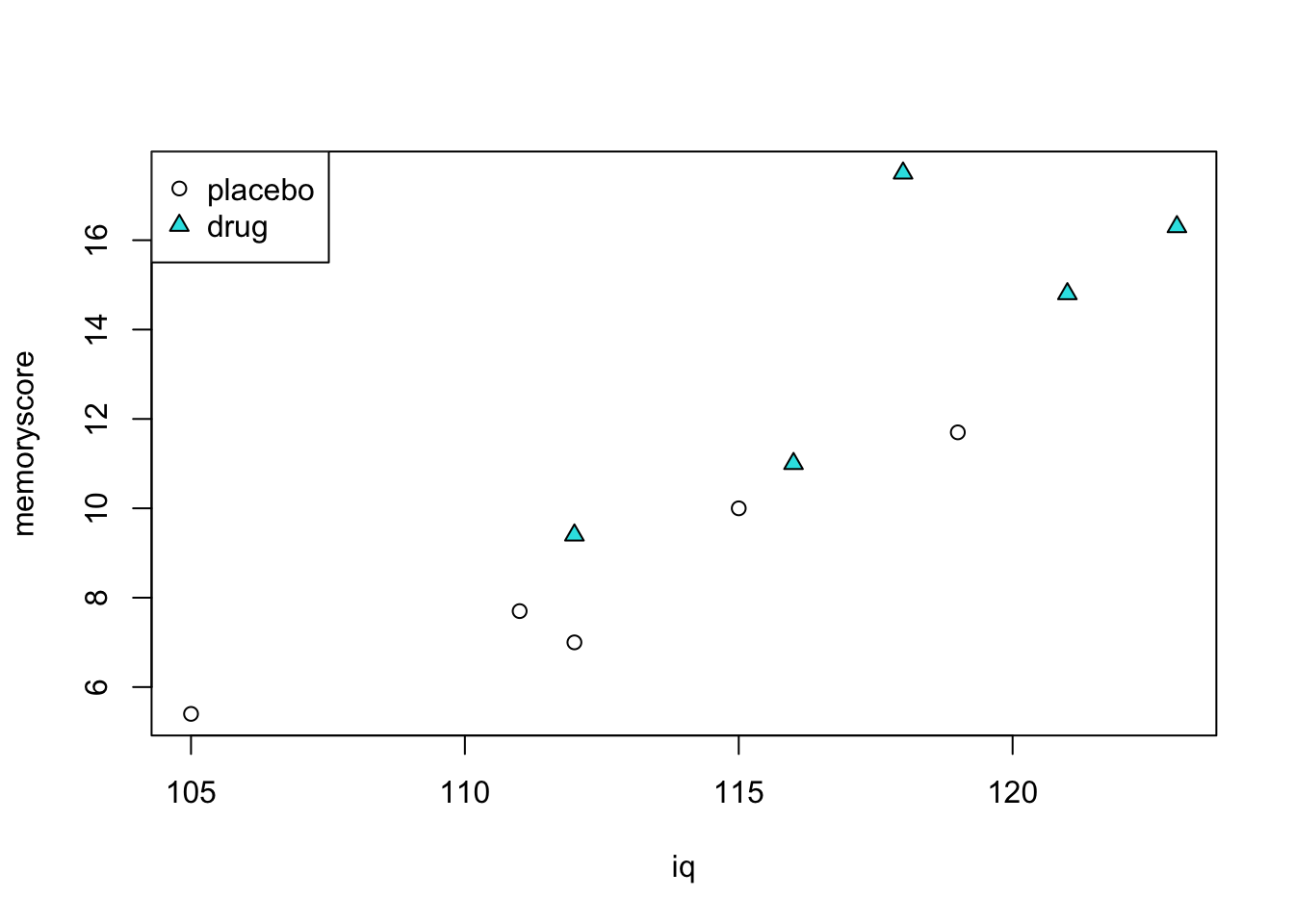
We can see three important things:
There seems to be a difference between groups on the dependent variable. Mean memory score for the placebo group is 8.4 and for the drug group is 13.8.
There is clearly a linear relationship between memory score and IQ.
The two groups also seem to differ on their IQ scores. Mean IQ for the placebo group is 112.4 and for the drug group is 118.
oneway ANOVA
If we were to run a simple one-way between subjects ANOVA, ignoring the covariate, we would get the following:
options(contrasts = c("contr.sum", "contr.poly"))
mod.1 <- aov(memoryscore ~ group)
summary(mod.1)
Df Sum Sq Mean Sq F value Pr(>F)
group 1 73.98 73.98 8.104 0.0216 *
Residuals 8 73.03 9.13
---
Signif. codes: 0 '***' 0.001 '**' 0.01 '*' 0.05 '.' 0.1 ' ' 1We would see that the omnibus test of the effect of group is significant at the 0.05 level (p = 0.0216). Make a note of the within-group variance. We can see that the error term in the ANOVA output (the Mean Sq value for the Residuals) is 9.13.
Note the first line of code above:
options(contrasts = c("contr.sum", "contr.poly"))We haven’t seen this before. It sets the default contrasts for factors in R to “sum-to-zero” contrasts. By using sum-to-zero contrasts, R codes a categorical variable (e.g. a Factor like group) as deviations from a grand mean. This is the default in many statistical software packages like SPSS and others. The contr.sum contrasts are the most intuitive and easiest to interpret. They are also the most general, and can be used for any number of levels of a factor. If you do not set the default contrasts to contr.sum, then R will use a different scheme, and your results will look different from what you expect. This is a common source of confusion for R users. There are other contrast schemes, like contr.treatment and contr.helmert, but they are not as general and are not as intuitive, and we will not be covering their use in this course.
Important: My advice is to always set the default contrasts to contr.sum at the beginning of every R script, using the line of code above, and then you won’t have to worry about it.
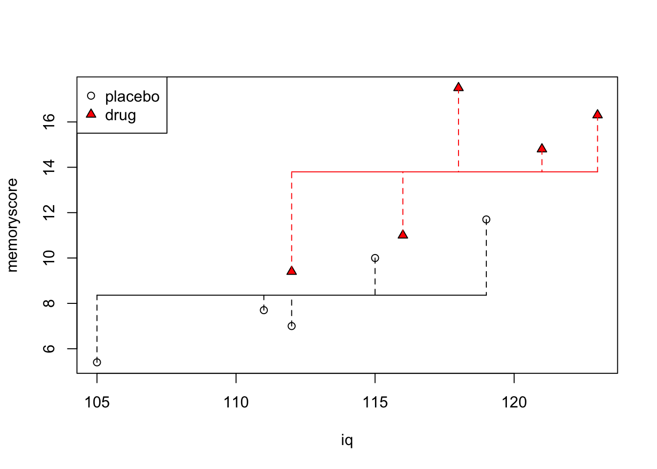
We can visualize our ANOVA model this way (see below): the horizontal line is the mean memory score of each group. The vertical dashed lines represent the error, under the full model.
Code
plot(iq,memoryscore, pch=c(rep(1,5),rep(24,5)), bg=c(rep(1,5),rep("red",5)))
legend("topleft", c("placebo","drug"), pch=c(1,24), pt.bg=c(1,"red"))
for (j in 1:2) {
    if (j==1) {
        w <- c(1,2,3,4,5)
        cl <- 1
    }
    if (j==2) {
        w <- c(6,7,8,9,10)
        cl <- "red"
    }
    lines(c(min(iq[w]),max(iq[w])), c(mean(memoryscore[w]),
        mean(memoryscore[w])), col=cl)
    for (i in 1:length(w)) {
        lines(c(iq[w[i]],iq[w[i]]), c(memoryscore[w[i]],
            mean(memoryscore[w])), lty=2, col=cl)
    }
}
Running an ANCOVA in R
The idea of ANCOVA then is to account for, i.e. model, the variation in memory score that can be captured by variation in IQ. This is done by modeling the relationship between memory score and IQ as a straight line. We can run the ANCOVA in the following way (see code snippet below), which is sort of neat, because we can explicitly state the full and restricted models as linear models using the lm() function, and then perform an F-test using the anova() function to compare each model.
Aside: the anova() function in R is a general function that can be used to compare any two models. It is not just for ANOVA. It can be used for comparing linear models, and other kinds of models as well. Here we can use the anova() function to compare the full and restricted models. It produces a test of whether term(s) in the full model that don’t appear in the restricted model are worth keeping in the model. The test it uses to assess this is an F-test.
mod.full <- lm(memoryscore ~ iq + group) # full model including covariate and group
mod.rest <- lm(memoryscore ~ iq)         # restricted model including only covariate
a2 <- anova(mod.rest, mod.full)          # F-test of full vs restricted models
print(a2)
Analysis of Variance Table
Model 1: memoryscore ~ iq
Model 2: memoryscore ~ iq + group
Res.Df RSS Df Sum of Sq F Pr(>F)
1 8 31.273
2 7 20.913 1 10.36 3.4678 0.1049I also show below that you can just use the anova() function on the full model alone, as well. In this case the row labelled group is the test of interest: i.e. the effect of group, after accounting for the covariate (i.e. with the covariate in the model). The row labelled iq is a test of the effect of the covariate itself, but this is not the main question we’re asking with ANCOVA.
The main question we’re asking with ANCOVA is: after accounting for the variance in memory score that can be explained by IQ, is there still a significant effect of group?
a3 <- anova(mod.full)
print(a3)
Analysis of Variance Table
Response: memoryscore
Df Sum Sq Mean Sq F value Pr(>F)
iq 1 115.743 115.743 38.7412 0.0004349 ***
group 1 10.360 10.360 3.4678 0.1048703
Residuals 7 20.913 2.988
---
Signif. codes: 0 '***' 0.001 '**' 0.01 '*' 0.05 '.' 0.1 ' ' 1You could also use the aov function we have used before. You get the same tests and the same output.
a3 <- aov(memoryscore ~ iq + group)
summary(a3)
Df Sum Sq Mean Sq F value Pr(>F)
iq 1 115.74 115.74 38.741 0.000435 ***
group 1 10.36 10.36 3.468 0.104870
Residuals 7 20.91 2.99
---
Signif. codes: 0 '***' 0.001 '**' 0.01 '*' 0.05 '.' 0.1 ' ' 1Notice how much lower our error term is (Mean Sq Residuals = 2.988) than before when we ran the ANOVA without the covariate.
Also notice that the effect of group is no longer significant! For the test of the effect of group, p = 0.105. This is important. It means that after we account for the differences in memory score that can be explained by differences in IQ, there is no longer a significant difference between the placebo and drug groups.
ANCOVA model coefficients
Graphically we can represent the ANCOVA full model by plotting the line corresponding to each pair of (\alpha_{j},\beta) for each group. Remember \alpha_{j} is the intercept and \beta is the (common) slope.
Code
plot(iq,memoryscore, pch=c(rep(1,5),rep(24,5)), bg=c(rep(1,5),rep("red",5)))
legend("topleft", c("placebo","drug"), pch=c(1,24), pt.bg=c(1,"red"))
mod.full.coef <- coef(mod.full)
print(mod.full.coef)
(Intercept) iq group1
-50.7033113 0.5363135 -1.2183223 Code
placebo.pred <- predict(mod.full)
for (j in 1:2) {
    if (j==1) {
        w <- c(1,2,3,4,5)
        cl <- 1
    }
    if (j==2) {
        w <- c(6,7,8,9,10)
        cl <- "red"
    }
    lines(c(min(iq[w]),max(iq[w])),
        c(min(placebo.pred[w]), max(placebo.pred[w])), col=cl)
}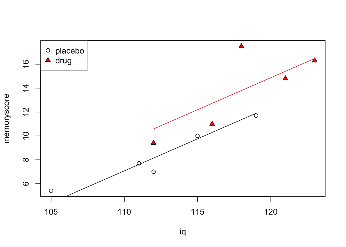
The coef() function gives us the model coefficients for mod.full, which is our full model (the output of the lm() function applied to our full model formula above).
The iq value (0.536) is the estimate of the slope of both lines, \beta in our equations above.
Note that in vanilla ANCOVA, the slopes of the lines in each group are the same. It is possible to estimate lines of different slopes in an ANCOVA model, but this is not the default. The default is to estimate a single slope for all groups.
The Intercept value (-50.703) is the value of \alpha_{1}, the intercept for the first level of the group factor, i.e. placebo. This is tricky and is an R gotcha: the group1 value (-1.218) is not equal to \alpha_{2}, but is what you have to add to \alpha_{1} in order to get the estimate of \alpha_{2}. Why is placebo the first level of the drug factor? Because we set it as such in the code at the top of these notes.
Thus \alpha_{2} = -50.703 + 0.536 = -50.167
Now, the test for the effect of group, is essentially a test of whether a full model that contains separate intercepts, \mu + \alpha_{j}, one for each level of the group factor (placebo, drug), is significantly better than a restricted model that only contains one intercept (in this case, since \alpha_{j} is missing from the model, so the intercept is simply \mu and since it doesn’t have a subscript j, is the same for each level of the group factor).
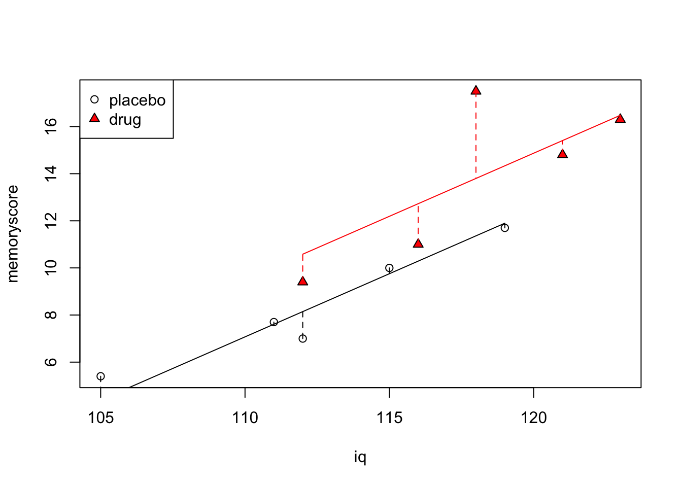
In the example above, the intercepts of the two lines corresponding to the full model (the values of \alpha_{1} and \alpha_{2}) are similar enough to each other that the restricted model probably fits the data just as well (indeed it does, according to the F-test we performed above).
Code
plot(iq,memoryscore, pch=c(rep(1,5),rep(24,5)), bg=c(rep(1,5),rep("red",5)))
legend("topleft", c("placebo","drug"), pch=c(1,24), pt.bg=c(1,"red"))
for (j in 1:2) {
    if (j==1) {
        w <- c(1,2,3,4,5)
        cl <- 1
    }
    if (j==2) {
        w <- c(6,7,8,9,10)
        cl <- "red"
    }
    lines(c(min(iq[w]),max(iq[w])),
        c(min(placebo.pred[w]), max(placebo.pred[w])), col=cl)
    for (i in 1:length(w)) {
        lines(c(iq[w[i]],iq[w[i]]),
            c(memoryscore[w[i]], placebo.pred[w[i]]), lty=2, col=cl)
    }
}
Adjusted Means
Having run an ANCOVA, and having estimated the relationship between IQ and memory score, we are now in a position to answer the interesting question, What would memory scores have been for placebo and drug groups IF their scores on IQ had been similar?. These are known as adjusted means.
Of course scores on IQ were not similar across groups, but ANCOVA allows us to answer the question, IF they had been similar, then taking account what we know about how memory score varies with IQ (independent of any experimental manipulation, like placebo vs drug), what would their scores have been?
We are going to ask R to generate predicted values of memory score given the full model that includes both \alpha_{j} and \beta parameters. We will then ask R to generate predictions of what memory score would have been, for both placebo and drug groups, if their scores on IQ had been the same. We will have to choose some arbitrary value of IQ, the usual is to simply choose the grand mean of IQ across both groups. We will use the predict() command to generate predictions from our full model.
First generate a data frame containing the grand mean of the covariate and the factor.
group.predict <- factor(     x = c("placebo","drug"),
                        levels = c("placebo","drug"))
iq.predict <- rep(mean(iq), 2)
data.predict <- data.frame(group=group.predict, iq=iq.predict)
print(data.predict)
group iq
1 placebo 115.2
2 drug 115.2Now use predict() to predict what memory score would have been for each group, if their scores on IQ had been the same.
adjmeans <- predict(mod.full, data.predict)
data.predict = data.frame(data.predict, memoryscore=adjmeans)
print(data.predict)
group iq memoryscore
1 placebo 115.2 9.861678
2 drug 115.2 12.298322So we see that our full model predicts that if the placebo and drug groups had been equal on IQ (for both groups, IQ = 115.2), then the mean memory score for the placebo group would have been 9.86 and for the drug group would have been 12.3. Compare that to the original unadjusted means (placebo = 8.36 and drug = 13.8) and you see that in this case, arithmetically adjusting for the group differences in IQ, resulted in less of a difference in memory score.
Graphically we can see how the prediction works, by drawing a vertical line at IQ = 115.2 and determining the value of memoryscore that intercepts that line for each group.
Code
plot(iq,memoryscore, pch=c(rep(1,5),rep(24,5)), bg=c(rep(1,5),rep("red",5)))
legend("topleft", c("placebo","drug"), pch=c(1,24), pt.bg=c(1,"red"))
for (j in 1:2) {
    if (j==1) {
        w <- c(1,2,3,4,5)
        cl <- 1
    }
    if (j==2) {
        w <- c(6,7,8,9,10)
        cl <- "red"
    }
    lines(c(min(iq[w]),max(iq[w])),
        c(min(placebo.pred[w]), max(placebo.pred[w])), col=cl)
    abline(v=mean(iq), lty=3, col="blue")
    abline(h=adjmeans[1], lty=2, col="black")
    abline(h=adjmeans[2], lty=2, col="red")
}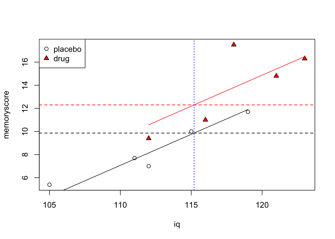
By including a covariate, you can change your conclusions in many ways (or fail to change them at all). An apparent effect can become weaker, or reversed, or be nullified altogether. An effect can become much stronger. Think about the conditions that must exist in your dataset for these different kinds of scenarios to happen.
Followup tests on individual means
After a significant omnibus test on the ANCOVA, you may wish to perform follow-up tests on individual means. Tests are done on adjusted means, in other words, on the modelled or assumed mean of each group if they had been equal on the covariate.
We can use the emmeans and rstatix packages to help with this. The emmeans package is a powerful tool for calculating and visualizing estimated marginal means, and the rstatix package is a powerful tool for calculating and visualizing post-hoc tests.
library(emmeans) # you may need to install.packages("emmeans") once
library(rstatix) # you may need to install.packages("rstatix") once
library(tidyverse)

memdata <- tibble(memoryscore, group, iq) # put our data into a tibble
mod.full <- lm(memoryscore ~ iq + group, data=memdata) # fit the full model
emmeans(mod.full, specs=~group) # calculate the estimated marginal means
group emmean SE df lower.CL upper.CL
placebo 9.86 0.853 7 7.85 11.9
drug 12.30 0.853 7 10.28 14.3
Confidence level used: 0.95 What’s shown above are the estimated memory score of each group, if they had been equal on the covariate (IQ). The estimated memory score for the placebo group is 9.86, and for the drug group is 12.3. These are the same values we calculated above using the predict() function.
To perform a follow-up pairwise tests on the adjusted means, we can use the emmeans_test() function from the rstatix package. Here we use the Holm correction for multiple comparisons.
emmeans_test(data            = memdata,
             formula         = memoryscore~group,
             covariate       = iq,
             p.adjust.method = "holm")
# A tibble: 1 × 9
term .y. group1 group2 df statistic p p.adj p.adj.signif
* <chr> <chr> <chr> <chr> <dbl> <dbl> <dbl> <dbl> <chr>
1 iq*group memoryscore placebo drug 7 -1.86 0.105 0.105 ns We see that the t-statistic is -1.86 with 7 df, and the p-value for the test is 0.105, which is far above a threshold of 0.05, so we fail to reject the null hypothesis that the adjusted means are the same.
What is the Meaning of Adjusted Means?
Although ANCOVA allows you to arithmetically adjust scores to predict what they would be if groups were equal on a covariate, if the fact of the matter is, in your experiment, they are not equal on the covariate, then it may be difficult to interpret the adjusted scores, in particular when your experiment involves a treatment of some kind. For example, in the fake data we have presented here on memory, drug vs placebo, and IQ, what if the drug in question actually has different effects on memory in low IQ versus high IQ individuals? The only way to truly deal with this problem is to equate the subjects on the covariate in the first place, prior to the treatment.
The adjusted means are produced by numerically interpolating, using the linear model, what the mean of the dependent variable would be for each group, if they had been equal on the covariate. Numerically adjusting the means may not be the same as controlling for the covariate. The only way to truly control for the covariate is to equate the groups on the covariate in the first place, prior to the treatment. This is the logic of a randomized controlled trial, where subjects are randomly assigned to groups, and the groups are equal on the covariate by the logic of random assignment.
ANCOVA Assumptions
Normality
Scores on the dependent variable must be normally distributed, and they must be so at all values of the covariate.
Like with one-way ANOVA we can use the Shapiro-Wilk test to test for normality of the residuals.
Homogeneity of Variance
The variance of the dependent variable must be the same for all levels of the factor, and it must be the same at all values of the covariate.
Like with one-way ANOVA we can use Levene’s test to test for homogeneity of variance.
Outliers
Like with one-way ANOVA, outliers can have a large effect on the results of an ANCOVA. You should always check for outliers and influential cases.
Homogeneity of Regression
The homogeneity of regression assumption is that the slope of the relationship between the dependent variable and the covariate is the same for all groups. In the equation for our full model this is apparent as \beta does not have a subscript (indicating different values for each group, i.e. each level of the factor).
Having said that, there is nothing stopping you from fitting a full model that has different slopes for each group. It would look like this:
Y_{ijk} = \mu + \beta_{j} X_{ij} + \alpha_{j} + \epsilon_{ijk}
The cost is, you lose a degree of freedom for every extra slope you have to estimate. In addition however, it would raise the troublesome question, why do different groups have different relationships between the dependent variable and the covariate? This may not be a problem. Then again it may be. It depends on the situation and the meaning of the dependent variable, the covariate, and the experimental design.
Incidentally, using the logic and tools we have developed already, you could perform a test to see if the slopes should be different very easily, by comparing the following two models:
\begin{array}{rll} \mathrm{full:} &Y_{ijk} &= \mu + \beta_{j} X_{ij} + \alpha_{j} + \epsilon_{ijk}\\ \mathrm{restricted:} &Y_{ijk} &= \mu + \beta X_{ij} + \alpha_{j} + \epsilon_{ijk} \end{array}
Look carefully and you see that the only difference between these two models is that the full model has a different slope for each group (\beta_{j}), and the restricted model has the same slope for each group (\beta, with no subscript _j).
To do this in R you could compare a full model that includes an interaction term of iq by group, with one that does not. In other words, in the full model, the effect of IQ on memory score (i.e. the slope) varies depending on the level of group (this is the definition of an interaction). In the restricted model, it does not.
mod.F <- lm(memoryscore ~ iq + group + iq:group)
mod.R <- lm(memoryscore ~ iq + group)
anova(mod.R, mod.F)
Analysis of Variance Table
Model 1: memoryscore ~ iq + group
Model 2: memoryscore ~ iq + group + iq:group
Res.Df RSS Df Sum of Sq F Pr(>F)
1 7 20.913
2 6 19.519 1 1.3943 0.4286 0.537The p-value of the F-test comparing these two models is 0.537, which is way above 0.05, which means we fail to reject the null hypothesis that the slopes are the same for each group. This is a good thing, because it means we can use the simpler model, which has more power (because we don’t have to “spend” our degrees-of-freedom on estimating different slopes for each group).
Or we could simply list the anova table for the full model:
anova(mod.F)Analysis of Variance Table
Response: memoryscore
Df Sum Sq Mean Sq F value Pr(>F)
iq 1 115.743 115.743 35.5788 0.0009948 ***
group 1 10.360 10.360 3.1848 0.1245828
iq:group 1 1.394 1.394 0.4286 0.5369540
Residuals 6 19.519 3.253
---
Signif. codes: 0 '***' 0.001 '**' 0.01 '*' 0.05 '.' 0.1 ' ' 1In this case the iq:group p-value is 0.537, just as above, indicating that the slopes are not reliably different across group.