Weekly homework assignments are comprised of two components: a Lab Component that your TA will guide you through in the weekly lab session, and a Home Component that you are to complete on your own. You must hand in both components. Both will count towards your grade.
Submit homework on OWL by 5:00 pm London ON time on the date shown in the Class Schedule.
Submit your homework assignment as a single RMarkdown file, using your last name and the homework assignment as a filename in the following format: gribble_n.Rmd where n is the homework assignment number.
Here is the R Markdown template file for this assignment: lastname_8.Rmd.
Lab Component
Experiments were carried out on six commercial goat farms to determine whether the standard worm drenching program was adequate. Forty goats were used in each experiment. Twenty of these, chosen at random, were drenched according to the standard program, while the remaining twenty were drenched more frequently. The goats were individually tagged and weighed at the start and end of the year-long study. For the first farm in the study the resulting live weight gains (gain), along with the initial live weights (wt), are given for the first farm in the study. In each experiment the main interest was in the comparison of the live weight gains between the two treatments (treatment).
1. Goats
Load the Goats dataset
options(contrasts=c("contr.sum","contr.poly")) # set contrasts to sum-to-zerolibrary(tidyverse)goats <-read_csv(url("https://www.gribblelab.org/2812_FW23/data/goats.csv"),col_types ="fnn")glimpse(goats)
Compute the mean and sd weight gain for each treatment group, and also report the number of observations in each group.
# A tibble: 2 × 4
  treatment mean_gain sd_gain     n
  <fct>         <dbl>   <dbl> <int>
1 standard       5.7     1.89    20
2 intensive      6.85    1.98    20
3. Graphics
Make a graphical plot showing the marginal means of weight gain (gain) by treatment (treatment).
4. ANOVA
Use simple one-way ANOVA to evaluate the effect of treatment (treatment) on weight gain (wt). Show the ANOVA table and interpret the results.
            Df Sum Sq Mean Sq F value Pr(>F)
treatment    1  13.23  13.225    3.52 0.0683 .
Residuals   38 142.75   3.757
---
Signif. codes:  0 '***' 0.001 '**' 0.01 '*' 0.05 '.' 0.1 ' ' 1
5. Linear Regression
Use linear regression to assess whether there is a linear relationship between weight gain (gain) and starting weight (wt).
Interpret the results—is there evidence of a linear relationship between weight gain and starting weight? What is the nature of the relationship?
Call:
lm(formula = gain ~ wt, data = goats)

Residuals:
    Min      1Q  Median      3Q     Max
-3.6566 -1.3214  0.1752  1.0082  3.6662

Coefficients:
            Estimate Std. Error t value Pr(>|t|)
(Intercept) 13.95675    1.77353   7.869 1.69e-09 ***
wt          -0.33182    0.07578  -4.379 9.03e-05 ***
---
Signif. codes:  0 '***' 0.001 '**' 0.01 '*' 0.05 '.' 0.1 ' ' 1

Residual standard error: 1.652 on 38 degrees of freedom
Multiple R-squared:  0.3354,    Adjusted R-squared:  0.3179
F-statistic: 19.18 on 1 and 38 DF,  p-value: 9.032e-05
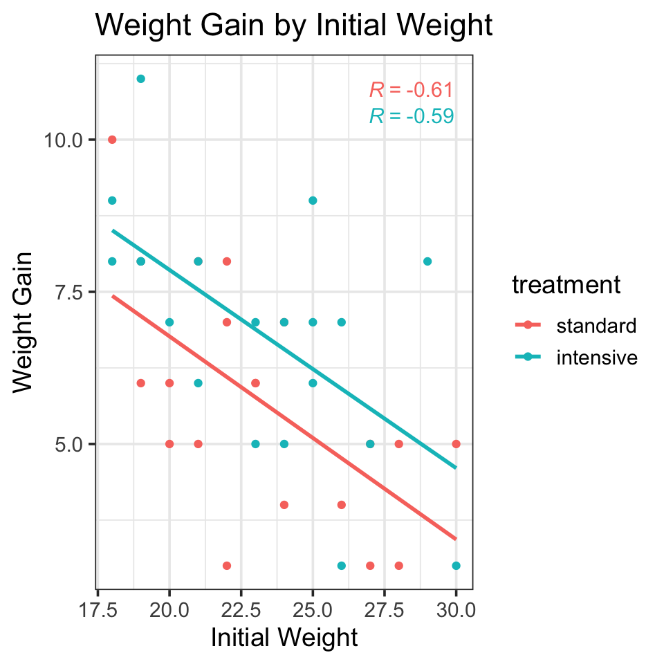
Generate a scatterplot of weight gain as a function of starting weight, showing the linear regression lines and the correlation coefficients separated by treatment group.
Interpret the plot. What does it tell you about the relationship between weight gain and starting weight, and how does this relationship appear to differ (or not) between the two treatment groups?
6. ANCOVA
Use ANCOVA to evaluate the effect of treatment (treatment) on weight gain (gain) while accounting for the linear association between weight gain and initial weight (wt). Interpret the results of the ANCOVA.
Calculate and show the raw means and the adjusted means of weight gain (gain) for each treatment group (treatment). Feel free to use either the predict() approach or the emmeans() approach to do this (as shown in the ANCOVA notes); either way is fine.
What is the conceptual difference between these two sets of means? Is there a substantial numerical difference between the two sets of means? Why or why not?
# A tibble: 2 × 3
  treatment mean_gain sd_gain
  <fct>         <dbl>   <dbl>
1 standard       5.7     1.89
2 intensive      6.85    1.98
Compare the outcome of the simple one-way ANOVA with the outcome of the ANCOVA. Explain why this happened in the context of (a) the raw means vs adjusted means, and (b) the relationship between weight gain and initial weight.
Home Component
You are Dean of the Faculty of Science. You have just met with one of the new Assistant Professors in the Department of Mathematics, for their annual performance evaluation. Professor X claims that their salary is much too low and they want you to give them a raise. They claim they are particularly good at teaching and thus deserves a raise. As evidence of this, they say that among the three sections of calculus taught in first year, their students (Section I) get the highest grades on the Calculus final exam, which is common to all three sections (see Table 1 below). You are the kind of Dean who likes to make decisions based on facts, and so you ask the Chair of the Department of Mathematics to gather some data for you. The Chair gives you final exam scores for a random sample of 50 students chosen from each of the three sections of Calculus 101.
9. Calculus Grades
Load in the dataset:
options(contrasts=c("contr.sum","contr.poly")) # set contrasts to sum-to-zerolibrary(tidyverse)calculus_data <-read_csv(url("https://www.gribblelab.org/2812_FW23/data/calculus1.csv"),col_types ="nnf")glimpse(calculus_data)
Rows: 150
Columns: 3
$ StudentID <dbl> 1, 2, 3, 4, 5, 6, 7, 8, 9, 10, 11, 12, 13, 14, 15, 16, 17, 1…
$ CalcGrade <dbl> 94, 81, 92, 81, 98, 77, 86, 76, 65, 80, 91, 90, 87, 94, 84, …
$ Section   <fct> I, I, I, I, I, I, I, I, I, I, I, I, I, I, I, I, I, I, I, I, …
Compute and show the mean and sd of Calculus grade for each of the three Calculus 101 sections, and report the number of observations in each section. Do the data suggest Professor X’s claim may be true or not?
10. ANOVA
Conduct a standard one-way ANOVA with follow-up tests (corrected for multiple comparisons) to assess whether the three sections differ in terms of final exam scores. What would you conclude based on the simple one-way ANOVA?
11. High School Grades
The Chair of the Mathematics Department calls you the next day and tells you that she also has available high-school mathematics grades for each of the students in the three sections of Calculus 101. She advises you that Section I (Professor X’s section) appears to contain a disproportionately high number of students from the same private school in Toronto, compared to sections II and III which contain a broader representation of students overall. She advises that you might want to take this information into consideration when comparing final grades in the three sections.
Rows: 150
Columns: 4
$ StudentID      <dbl> 1, 2, 3, 4, 5, 6, 7, 8, 9, 10, 11, 12, 13, 14, 15, 16, …
$ CalcGrade      <dbl> 94, 81, 92, 81, 98, 77, 86, 76, 65, 80, 91, 90, 87, 94,…
$ Section        <fct> I, I, I, I, I, I, I, I, I, I, I, I, I, I, I, I, I, I, I…
$ HighSchoolMath <dbl> 72, 83, 83, 80, 97, 82, 80, 76, 68, 74, 86, 86, 87, 66,…
Compute and show the mean and sd of Calculus grade and the mean and sd of High School Math grade for each of the three Calculus 101 sections, and report the number of observations in each section. What do the High School Math grades suggest about the three sections of Calculus 101, and how might this information be relevant to Professor X’s claim?
Using a one-way ANOVA with appropriate follow-up tests, assess whether the average high-school math grades differ between the three sections of Calculus 101. Interpret the results.
Fit a linear model to assess whether there appears to be a linear relationship between High School Math grades (HighSchoolMath) and grades in Calculus 101 (CalcGrade). Interpret the results.
Generate a scatterplot of calculus grade as a function of high school math, showing the linear regression lines and the correlation coefficients, separated by calculus section.
12. ANCOVA
Conduct an ANCOVA in which you take into account the high-school grades of students and re-assess whether there is a statistically reliable difference between Calculus grades across the three sections. Report adjusted means and regardless of the outcome of the ANCOVA, perform follow-up tests and interpret them.
Based on the ANCOVA results, what can you conclude about the final exam scores from Sections I, II and III of Calculus 101?
What can you conclude about Professor X’s claim? Would you give them a raise based on your ANCOVA analysis? Why or why not?