  mpg cylinders displacement horsepower weight acceleration year origin
1  18         8          307        130   3504         12.0   70      1
2  15         8          350        165   3693         11.5   70      1
3  18         8          318        150   3436         11.0   70      1
4  16         8          304        150   3433         12.0   70      1
5  17         8          302        140   3449         10.5   70      1
6  15         8          429        198   4341         10.0   70      1
                       name
1 chevrolet chevelle malibu
2         buick skylark 320
3        plymouth satellite
4             amc rebel sst
5               ford torino
6 ford galaxie 500Homework 3
Psychology 2812B FW23
Weekly homework assignments are comprised of two components: a Lab Component that your TA will guide you through in the weekly lab session, and a Home Component that you are to complete on your own. You must hand in both components. Both will count towards your grade.
Submit homework on OWL by 5:00 pm London ON time on the date shown in the Class Schedule.
Submit your homework assignment as a single RMarkdown file, using your last name and the homework assignment as a filename in the following format: gribble_n.Rmd where n is the homework assignment number.
Here is the R Markdown template file for this assignment: lastname_3.Rmd.
Lab Component
1. ISLR2 Auto dataset
Load the tidyverse.
Install and load the ISLR2 package and inspect the dataset called Auto:
2. Plot car’s weight versus fuel efficiency
Plot each car’s weight (pounds) against its fuel efficiency (mpg) (miles per gallon of fuel) and overlay a linear fit using geom_smooth(method="lm", se=FALSE):
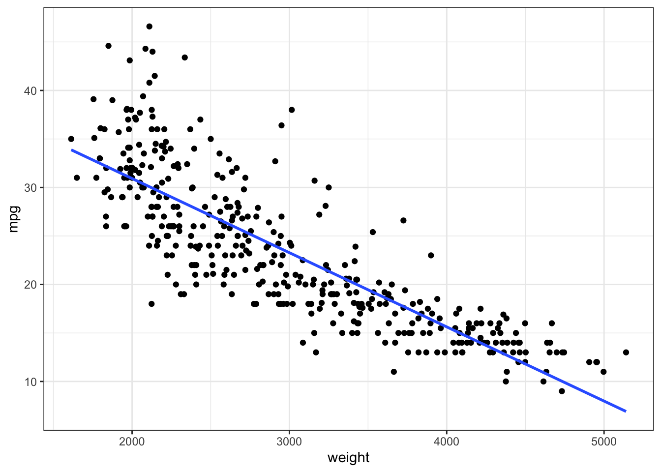
3. Correlation coefficient
Compute the correlation (Pearson’s R) between weight and mpg:
[1] -0.83224424. Re-plot with R shown on Figure
Re-plot the data and show the correlation coefficient on the plot.
Hint: the stat_correlation() function in the ggpmisc package can do this easily (you may have to install.packages("ggpmisc")).
Hint2: you can also add a line using the stat_poly_line(se=FALSE) function (or you can do like before and use the geom_smooth(method="lm", se=FALSE) function, your choice):

5. Goodness of fit: R^{2}
We are interested in predicting the fuel efficiency of cars (mpg, miles per gallon) from their weight (pounds). In the previous assignment we fit a linear regression model to predict mpg from weight.
Report the R^{2} value for the goodness of fit of the regression model. Note you can extract this from the summary() of your lm() model, it’s called r.squared.
[1] 0.6926304Write a sentence about what this value of R^{2} means in the context of prediction.
6. Goodness of fit: s_{est}
Report the standard error of the estimate s_{est} of the regression model. Note you can extract this from the summary() of your lm() model, it’s called sigma.
[1] 4.332712Write a sentence about what this value of R^{2} means (hint: variance accounted for).
7. Confidence intervals
Compute the 95% confidence intervals for the regression coefficients (intercept and slope) in your regression model. You can do this by hand using the formula,
or
you can use the confint() function, just feed it two things, first your regression model (object=mymod, assuming you named your regression model mymod), and second, the confidence level you want (level=95%).
                   2.5 %      97.5 %
(Intercept) 44.646282308 47.78676679
weight      -0.008154515 -0.00714017
Write a sentence about what these confidence intervals mean.
Home Component
8. Interpretation & Inference
Write a sentence or two describing the relationship between weight and mpg. Say something about the strength and the direction of the correlation.
Conduct a significance test of the correlation between weight and mpg using cor.test().
Check the normality assumption using shapiro.test().
Report the results of your tests.
If the normality assumption is violated, re-do the correlation significance test using Spearman’s rank correlation and report the results.
Based on your work so far write a sentence or two about whether you think a linear relationship exists (or not) and why (or why not).
9. Linear Regression model
Compute a linear regression model in which you predict mpg from weight. Use the lm() function in R to define your model. Then use the summary() function to display information about your regression model.
10. Model coefficients
What is the Y-intercept of your regression line?
What is the slope of your regression line?
Write a sentence that explains the meaning of the slope.
11. Significance tests
Report the results of the significance test on the model as a whole. Report the F-statistic, the degrees of freedom, and the p-value. Write sentences for each, e.g. “The F-statistic is ___“.
Hint: this information is given when you execute the summary() command and feed it the name of your lm() object, e.g. summary(mymod) assuming you named your lm() model object mymod.
Write a sentence to say what the p-value means. Specifically, say what this is the probability of. Be precise in your language. If you mention the null hypothesis, be precise about what the null hypothesis is.
Also report the p-values for each of the model coefficients (intercept, slope). Also write a sentence to say what each of these p-values mean. Each of them is the probability of what precisely? Say what the null hypotheses are for each p-value test.
12. Model prediction
Using your regression model, predict the fuel efficiency in mpg of a car whose weight is 2000 pounds. Note you can do this by hand using the model coefficients from above,
or
you can use the predict.lm() function in R to do it. Type ?predict.lm on the console to view the help documentation. You just feed it two arguments: first, your lm() model object, and second, a tibble containing a value for the predictor variable weight (e.g. tibble(weight=2000)) and it uses the model to predict the corresponding value of the predicted variable mpg.
Either of the two above methods is acceptable.
Write a sentence that explains what this number means.
13. Does mpg improve over the years?
Using your knowledge of the functionality within dplyr and ggplot2 packages, repeat the plot from Question 4 above, but plot two separate geom_smooth() lines, one for each of two subsets of the cars: (1) for “older” cars with model years between (and including) 1970, 1971, and 1972, and (2) for “newer” cars with model years 1980, 1981, 1982. Hint: remember you can add a color=___ argument to the aes() mapping argument to separate out geoms by color.
Hint: Before you generate your ggplot, you can use the filter() function from dplyr to create a new tibble that includes only older and newer cars according to the definition above. Then you could add a new variable to the tibble called age (using mutate()) that has a value of "older" if the year is <=72 and "newer" if the year is >=80. Then you could use the option color=age in your ggplot aes() mapping.
Or of course you could do it in many other ways of your choosing.
Code
oldcars <- Auto %>% filter(year <= 72) %>% mutate(age="older")
newcars <- Auto %>% filter(year >= 80) %>% mutate(age="newer")
Auto2 <- bind_rows(oldcars, newcars)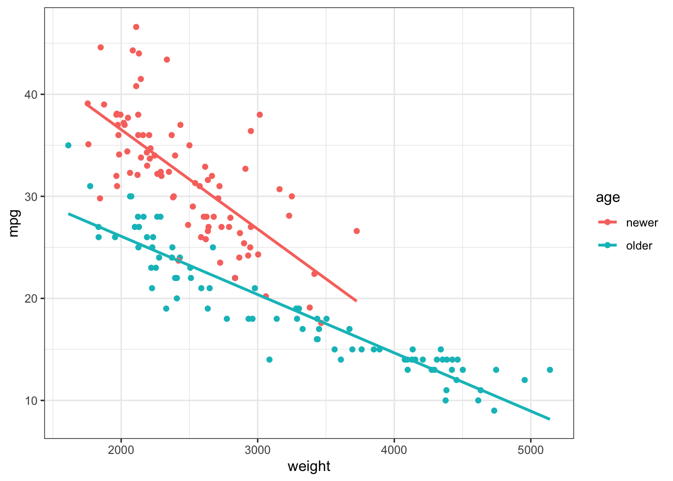
14. Regression models
Fit two regression models predicting mpg from weight, one for “older” cars and one for “newer” cars as defined above.
Report the y-intercept for “older” and “newer” cars.
Report the slope for “older” and “newer” cars.
Write a sentence or two about what a difference in slope and intercept between older and newer cars might mean in the context of the relationship between weight and fuel efficiency.
Answer the following question: based only on the regression lines in the plot above and the differences in slope and intercept, is there anything that we can actually conclude about whether fuel efficiency actually improved over the years? Explain your answer. Hint: remember our discussions about randomness and what the null hypothesis is, and about the difference between a sample and a population.