Factorial ANOVA: follow-up tests

Week 10

Example Data

• fictitious blood pressure drug trial
• DV is bloodpressure (lower is better)
• IVs: biofeedback (2 levels) and drug (3 levels)

library(tidyverse)
bpdata <- read_csv(url("https://www.gribblelab.org/2812/data/bpdata2.csv"),
                   col_types="nff")
bpdata

# A tibble: 30 × 3
   bloodpressure biofeedback drug   
           <dbl> <fct>       <fct>  
 1           188 present     absent 
 2           183 present     absent 
 3           198 present     absent 
 4           179 present     absent 
 5           193 present     absent 
 6           186 absent      present
 7           191 absent      present
 8           190 absent      present
 9           181 absent      present
10           176 absent      present
# ℹ 20 more rows

Code

bpdata_means <- bpdata %>%
  group_by(biofeedback, drug) %>%
  summarise(meanbp = mean(bloodpressure),
            se     = sd(bloodpressure)/sqrt(n()),
            n      = n())
bpdata_means

# A tibble: 6 × 5
# Groups:   biofeedback [2]
  biofeedback drug     meanbp    se     n
  <fct>       <fct>     <dbl> <dbl> <int>
1 present     absent     188.  3.40     5
2 present     present    168.  3.83     5
3 present     highdose   162.  5.40     5
4 absent      absent     190   3.54     5
5 absent      present    185.  2.82     5
6 absent      highdose   185.  1.52     5

Code

bp.plot <- 
ggplot(data=bpdata_means,
       mapping = aes(x = drug, 
                     y = meanbp, 
                     color = biofeedback)) + 
  geom_point(pch = 15, 
             size = 2) +
  geom_line(aes(group = biofeedback)) +
  geom_errorbar(aes(ymin = meanbp-se,
                    ymax = meanbp+se), 
                width=.1) +
  geom_jitter(data = bpdata,
              mapping = aes(x = drug, y = bloodpressure),
              width = 0.1,
              alpha = 0.5) +
  labs(title = "Blood Pressure Experiment",
       x = "Drug",
       y = "Blood Pressure",
       color = "biofeedback") +
  theme_bw(base_size=14)
set.seed(2812)
bp.plot

Example Data

• we conducted a 2-way factorial ANOVA

my.anova <- aov(bloodpressure ~ biofeedback * drug,
                data = bpdata)
summary(my.anova)

                 Df Sum Sq Mean Sq F value   Pr(>F)
biofeedback       1 1442.2  1442.2  22.150 8.76e-05
drug              2 1401.8   700.9  10.765  0.00046
biofeedback:drug  2  607.3   303.6   4.664  0.01945
Residuals        24 1562.6    65.1                 

• significant main effect of biofeedback,
  F(1,24)=22.15, p=8.76e-05
• significant main effect of drug,
  F(2,24)=10.77, p=.00046
• significant biofeedback x drug interaction,
  F(2,24)=4.66, p=.01945

• what are our next steps?

2x2 ANOVA Follow-up Tests

• If A x B interaction is not significant—follow up main effects
  • is main effect of A significant?
    • Yes: conduct pairwise post-hoc tests for marginal means of A
    • No: do nothing
  • is main effect of B significant?
    • Yes: conduct pairwise post-hoc tests for marginal means of B
    • No: do nothing

2x2 ANOVA Follow-up Tests

• If A x B interaction is significant:
  • test the simple main effect of A within each level of B
  • (or if you prefer, the simple main effect of B within each level of A)
  • like doing a series of one-way ANOVAs on A, one for each level of B
• for each simple main effect that is significant,
  • conduct pairwise post-hoc tests on levels of A within that level of B

2x2 ANOVA Follow-up Tests

• sometimes researchers bypass the simple main effects tests
  • go directly to pairwise post-hoc tests to investigate the interaction effect
• There are differing opinions on whether this is ok
  • some say it is not ok, because the simple main effects are there to protect against Type-I error
  • others say it is ok, as long as the pairwise posthoc tests are properly corrected for Type-I error

2x2 ANOVA Follow-up Tests

• let’s assume for now that if there is a significant interaction effect,
  • we will do simple main effects tests first
  • then pairwise post-hoc tests on the significant simple main effects
• let’s look at some examples of different scenarios

Example 1

Example 2

Example 3

Example 3

Example 3

Example 3

Example 3

Example 3

Following up a Main Effect in R

                 Df Sum Sq Mean Sq F value   Pr(>F)
biofeedback       1 1442.2  1442.2  22.150 8.76e-05
drug              2 1401.8   700.9  10.765  0.00046
biofeedback:drug  2  607.3   303.6   4.664  0.01945
Residuals        24 1562.6    65.1                 

• for purposes of demonstration let’s pretend for now that the biofeedback x drug interaction is not significant
• let’s follow up the main effect of drug
• marginal means for the Drug factor:

library(emmeans)
(drugMM <- emmeans(my.anova, specs = ~ drug))

 drug     emmean   SE df lower.CL upper.CL
 absent      189 2.55 24      184      194
 present     177 2.55 24      171      182
 highdose    173 2.55 24      168      178

Results are averaged over the levels of: biofeedback 
Confidence level used: 0.95 

pairs(drugMM, adjust="tukey")

 contrast           estimate   SE df t.ratio p.value
 absent - present       12.5 3.61 24   3.464  0.0055
 absent - highdose      15.9 3.61 24   4.406  0.0005
 present - highdose      3.4 3.61 24   0.942  0.6199

Results are averaged over the levels of: biofeedback 
P value adjustment: tukey method for comparing a family of 3 estimates 

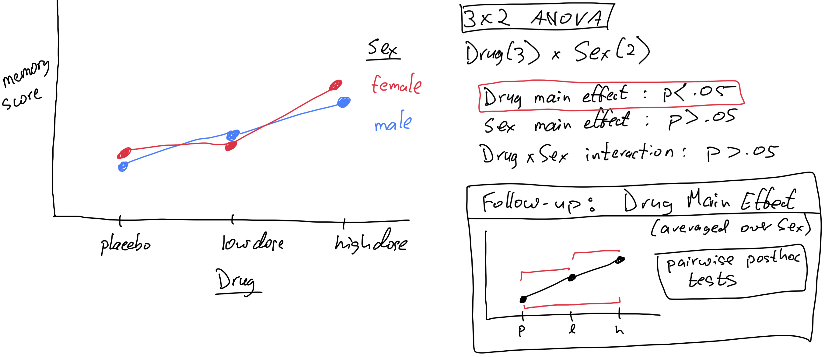
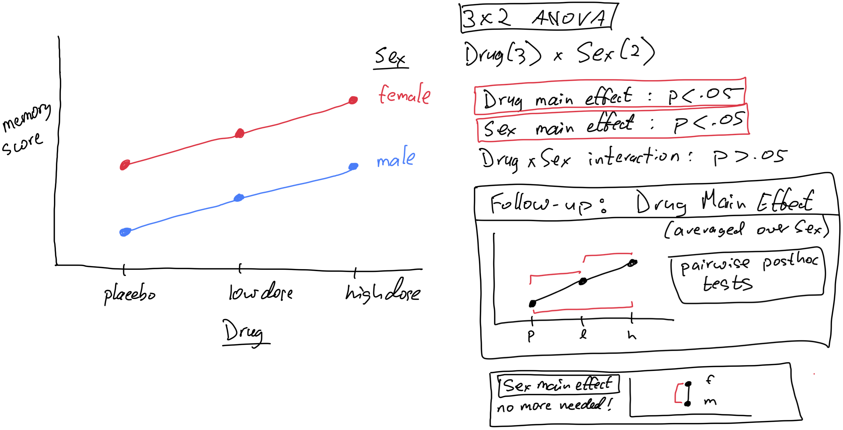
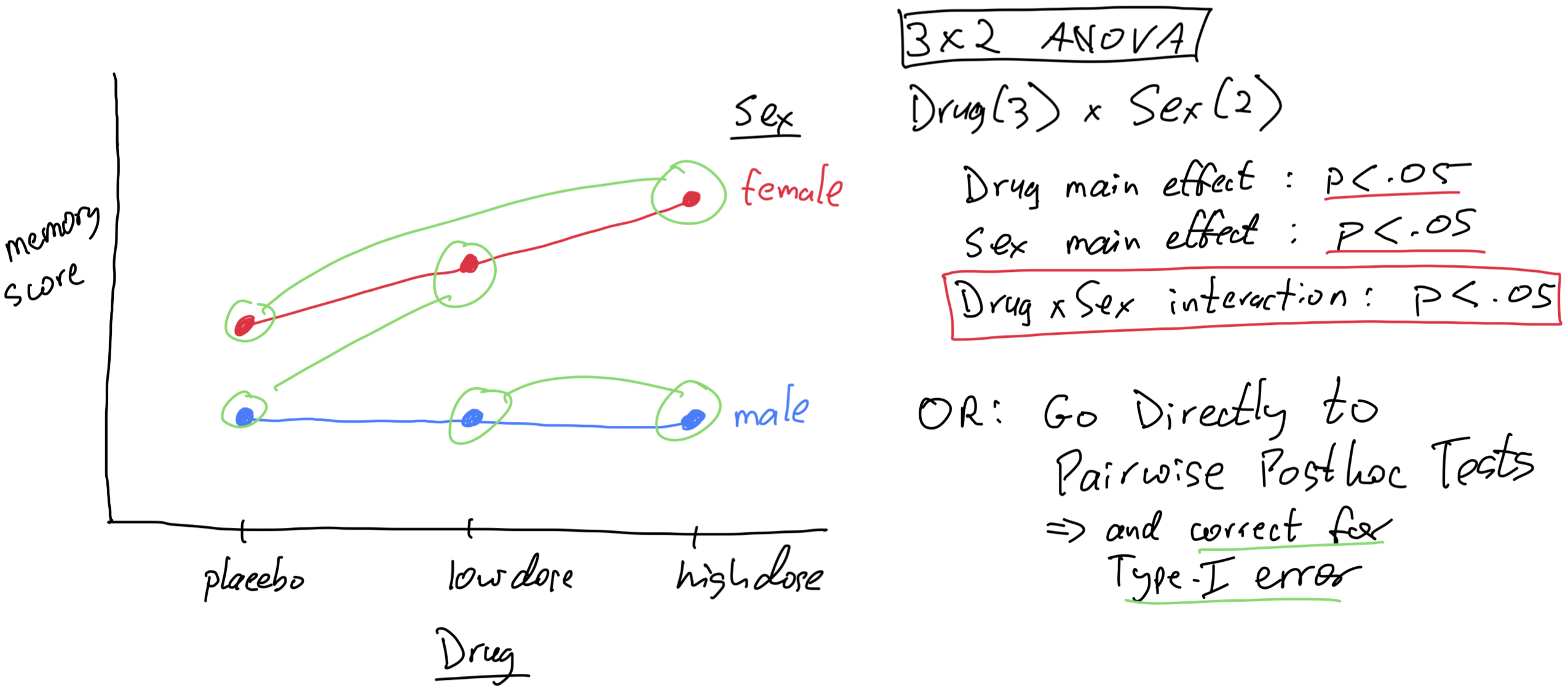
Following up a Main Effect in R

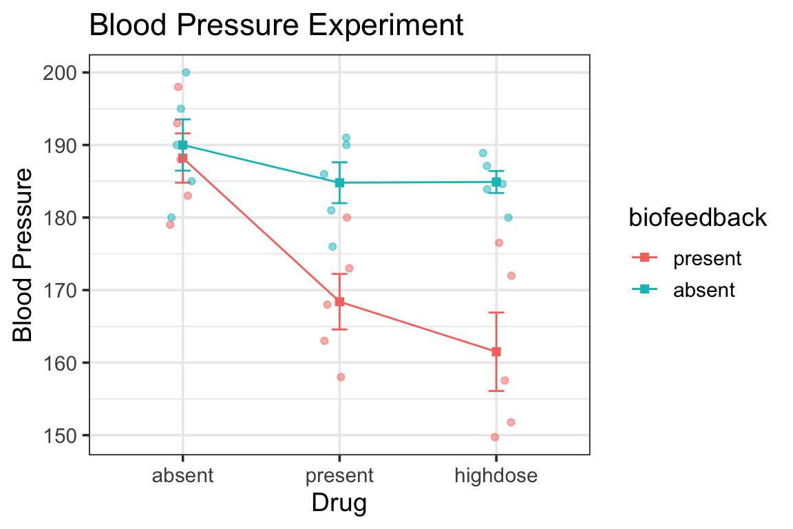
                 Df Sum Sq Mean Sq F value   Pr(>F)
biofeedback       1 1442.2  1442.2  22.150 8.76e-05
drug              2 1401.8   700.9  10.765  0.00046
biofeedback:drug  2  607.3   303.6   4.664  0.01945
Residuals        24 1562.6    65.1                 

• for purposes of demonstration let’s pretend for now that the biofeedback x drug interaction is not significant
• let’s follow up the main effect of drug
• marginal means for the Drug factor:

library(emmeans)
(drugMM <- emmeans(my.anova, specs = ~ drug))

 drug     emmean   SE df lower.CL upper.CL
 absent      189 2.55 24      184      194
 present     177 2.55 24      171      182
 highdose    173 2.55 24      168      178

Results are averaged over the levels of: biofeedback 
Confidence level used: 0.95 

pairs(drugMM, adjust="holm")

 contrast           estimate   SE df t.ratio p.value
 absent - present       12.5 3.61 24   3.464  0.0040
 absent - highdose      15.9 3.61 24   4.406  0.0006
 present - highdose      3.4 3.61 24   0.942  0.3558

Results are averaged over the levels of: biofeedback 
P value adjustment: holm method for 3 tests 

Following up a Main Effect in R

                 Df Sum Sq Mean Sq F value   Pr(>F)
biofeedback       1 1442.2  1442.2  22.150 8.76e-05
drug              2 1401.8   700.9  10.765  0.00046
biofeedback:drug  2  607.3   303.6   4.664  0.01945
Residuals        24 1562.6    65.1                 

• for purposes of demonstration let’s pretend for now that the biofeedback x drug interaction is not significant
• let’s follow up the main effect of biofeedback
• marginal means for the biofeedback factor:

library(emmeans)
(biofeebdackMM <- emmeans(my.anova, specs = ~ biofeedback))

 biofeedback emmean   SE df lower.CL upper.CL
 present        173 2.08 24      168      177
 absent         187 2.08 24      182      191

Results are averaged over the levels of: drug 
Confidence level used: 0.95 

• we don’t need any more tests, since there are only 2 groups
• we can simply refer to the F test of biofeedback in the ANOVA table

Following up a Main Effect in R

                 Df Sum Sq Mean Sq F value   Pr(>F)
biofeedback       1 1442.2  1442.2  22.150 8.76e-05
drug              2 1401.8   700.9  10.765  0.00046
biofeedback:drug  2  607.3   303.6   4.664  0.01945
Residuals        24 1562.6    65.1                 

• for purposes of demonstration let’s pretend for now that the biofeedback x drug interaction is not significant
• let’s follow up the main effect of biofeedback
• marginal means for the biofeedback factor:

library(emmeans)
(biofeebdackMM <- emmeans(my.anova, specs = ~ biofeedback))

 biofeedback emmean   SE df lower.CL upper.CL
 present        173 2.08 24      168      177
 absent         187 2.08 24      182      191

Results are averaged over the levels of: drug 
Confidence level used: 0.95 

• BTW: an F-test with 1 numerator df is equivalent to a t-test
• F = t^{2}
• F(1,24)=22.15 is equivalent to t(24)=4.71

Following up an Interaction in R

                 Df Sum Sq Mean Sq F value   Pr(>F)
biofeedback       1 1442.2  1442.2  22.150 8.76e-05
drug              2 1401.8   700.9  10.765  0.00046
biofeedback:drug  2  607.3   303.6   4.664  0.01945
Residuals        24 1562.6    65.1                 

• we will test the simple main effect of drug for each level of biofeedback
• within “Absent” biofeedback:

bpdata_absent <- bpdata %>%
                 filter(biofeedback == "absent")
absent.anova  <- aov(bloodpressure ~ drug,
                     data = bpdata_absent)
summary(absent.anova)

            Df Sum Sq Mean Sq F value Pr(>F)
drug         2   88.4    44.2   1.166  0.345
Residuals   12  454.8    37.9               

• no simple main effect in “Absent”, F(2,12)=1.17, p=0.345

Following up an Interaction in R

                 Df Sum Sq Mean Sq F value   Pr(>F)
biofeedback       1 1442.2  1442.2  22.150 8.76e-05
drug              2 1401.8   700.9  10.765  0.00046
biofeedback:drug  2  607.3   303.6   4.664  0.01945
Residuals        24 1562.6    65.1                 

• we will test the simple main effect of drug for each level of biofeedback
• within “Present” biofeedback:

bpdata_present <- bpdata %>%
                  filter(biofeedback == "present")
present.anova  <- aov(bloodpressure ~ drug,
                      data = bpdata_present)
summary(present.anova)

            Df Sum Sq Mean Sq F value Pr(>F)
drug         2   1921   960.3    10.4 0.0024
Residuals   12   1108    92.3               

• yes simple main effect in “Present”, F(2,12)=10.4, p=.0024
• now we need to follow up the simple main effect of drug in biofeedback “Present”

Following up an Interaction in R

                 Df Sum Sq Mean Sq F value   Pr(>F)
biofeedback       1 1442.2  1442.2  22.150 8.76e-05
drug              2 1401.8   700.9  10.765  0.00046
biofeedback:drug  2  607.3   303.6   4.664  0.01945
Residuals        24 1562.6    65.1                 

• simple main effect of drug within biofeedback present:

bpdata_present <- bpdata %>%
                  filter(biofeedback == "present")
present.anova  <- aov(bloodpressure ~ drug,
                      data = bpdata_present)
summary(present.anova)

            Df Sum Sq Mean Sq F value Pr(>F)
drug         2   1921   960.3    10.4 0.0024
Residuals   12   1108    92.3               

• drug marginal means: biofeedback present

(drugSME <- emmeans(present.anova, specs = ~ drug))

 drug     emmean  SE df lower.CL upper.CL
 absent      188 4.3 12      179      198
 present     168 4.3 12      159      178
 highdose    162 4.3 12      152      171

Confidence level used: 0.95 

pairs(drugSME, adjust="holm")

 contrast           estimate   SE df t.ratio p.value
 absent - present       19.8 6.08 12   3.258  0.0137
 absent - highdose      26.7 6.08 12   4.394  0.0026
 present - highdose      6.9 6.08 12   1.135  0.2785

P value adjustment: holm method for 3 tests 

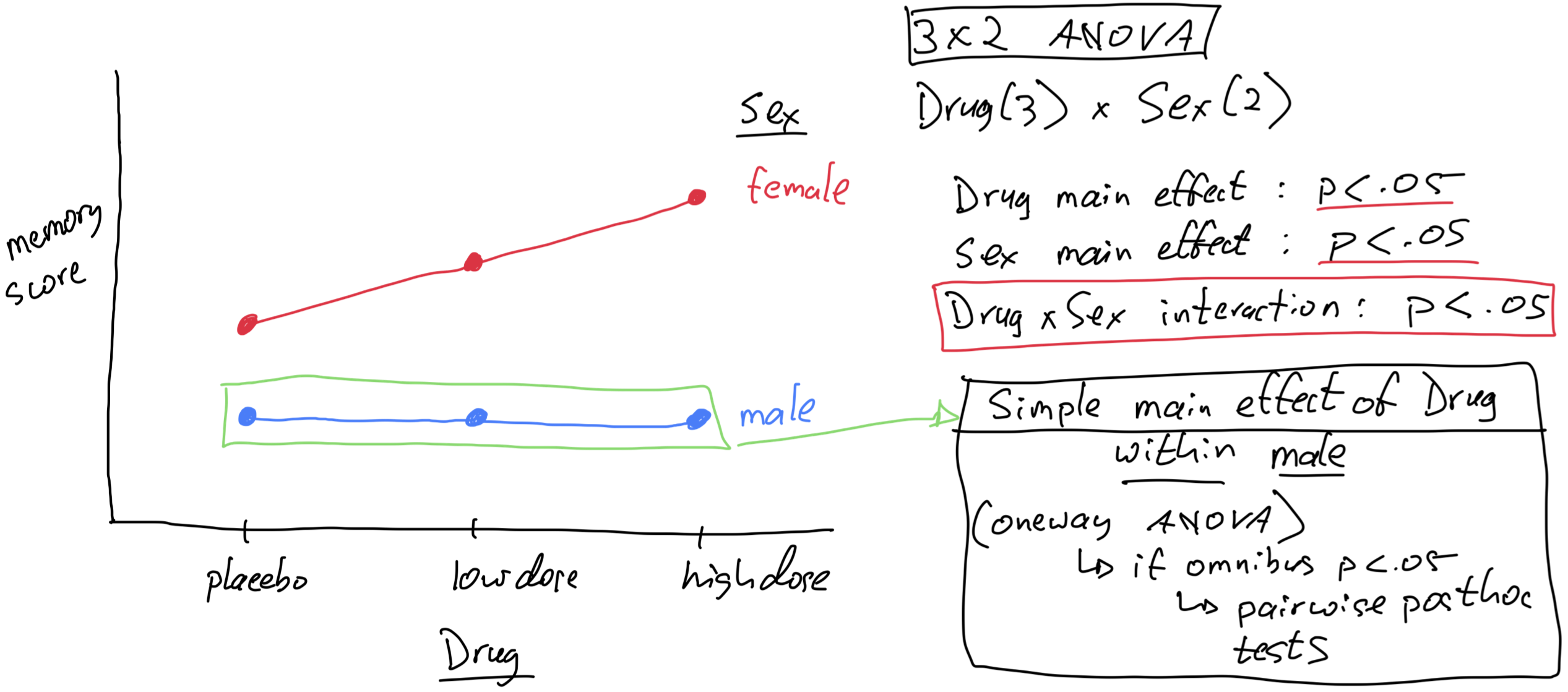
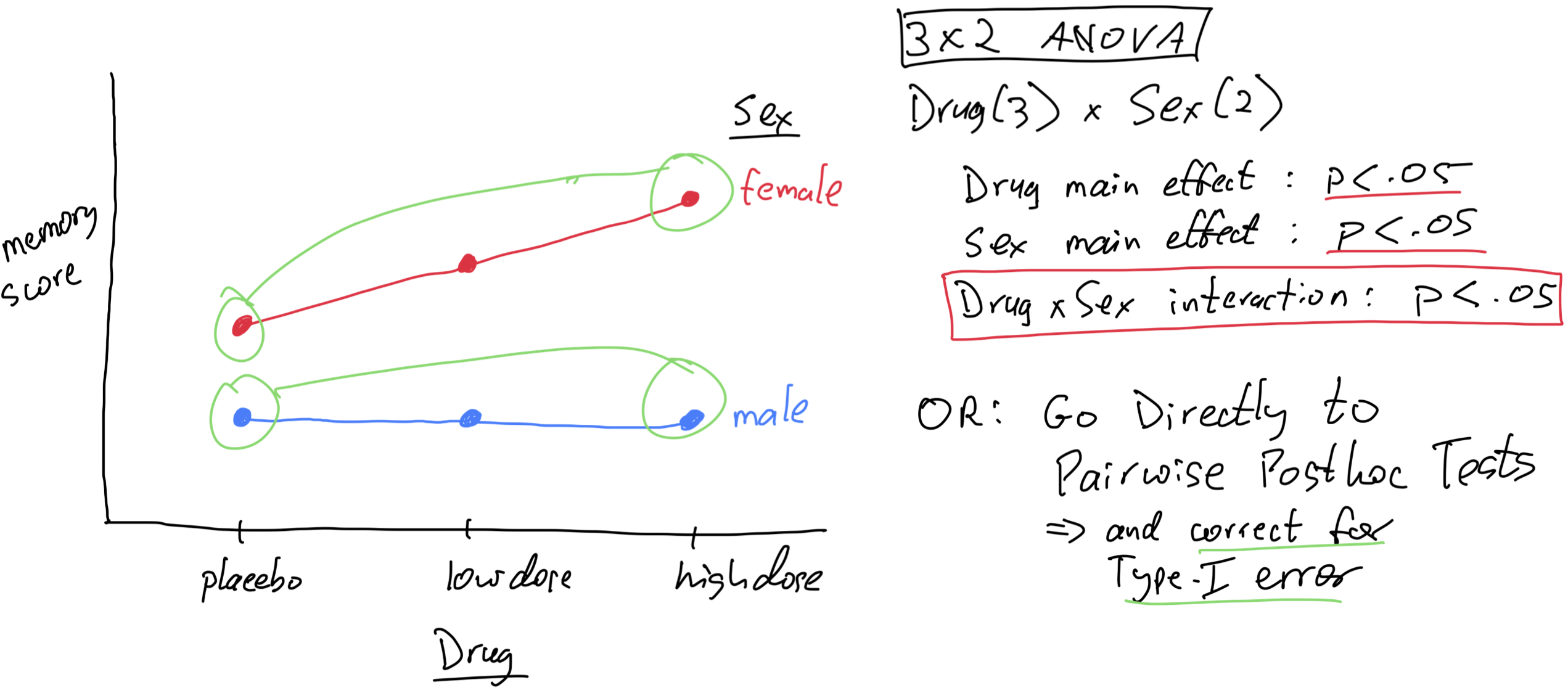
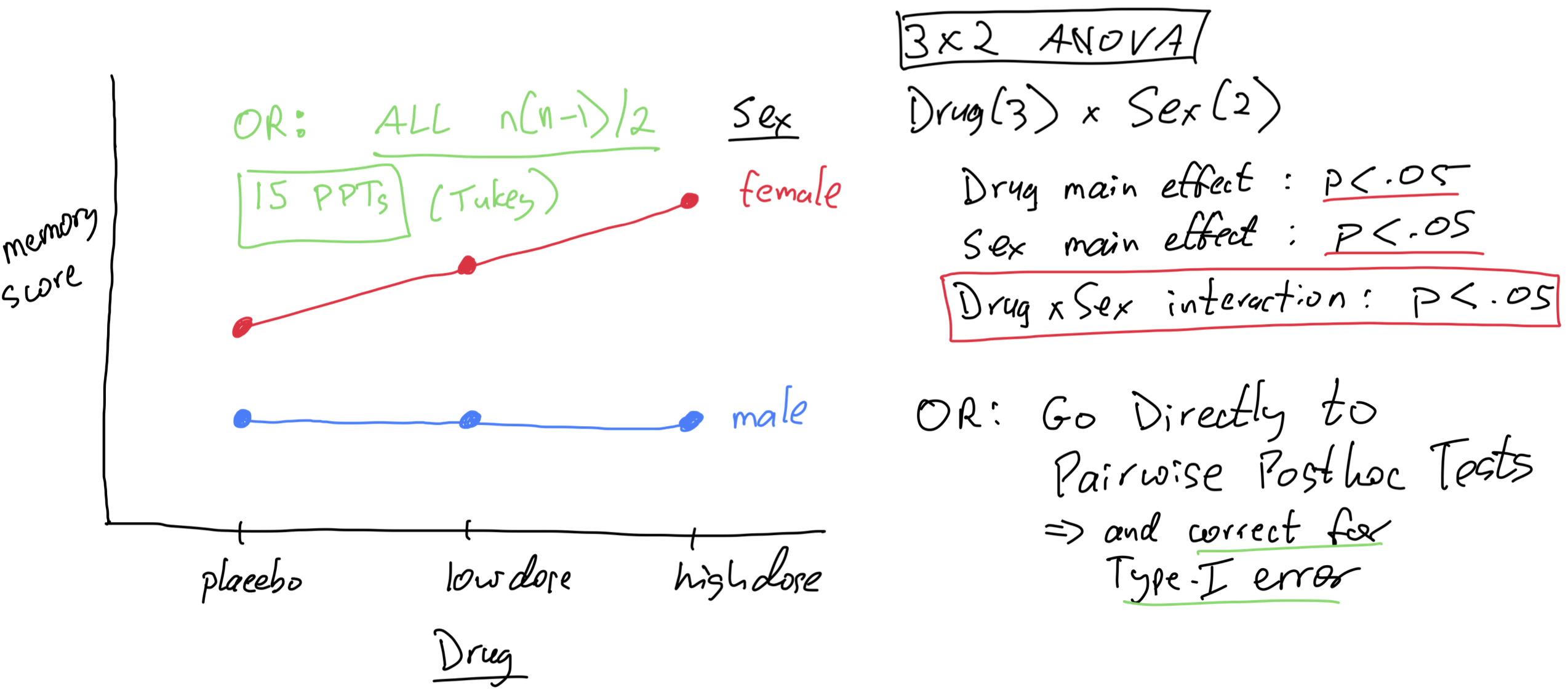
Following up an Interaction in R

• notice the ANOVA tables for the full ANOVA and for the simple main effect test:

summary(my.anova)

                 Df Sum Sq Mean Sq F value   Pr(>F)
biofeedback       1 1442.2  1442.2  22.150 8.76e-05
drug              2 1401.8   700.9  10.765  0.00046
biofeedback:drug  2  607.3   303.6   4.664  0.01945
Residuals        24 1562.6    65.1                 

summary(present.anova)

            Df Sum Sq Mean Sq F value Pr(>F)
drug         2   1921   960.3    10.4 0.0024
Residuals   12   1108    92.3               

• error term (Residuals) for full ANOVA is smaller than for simple main effect test
• the Residuals df is way larger because it uses the whole dataset
• the full ANOVA Residuals is also a more accurate estimate since it uses more data—it’s a pooled estimate of within-group variability

• some researchers prefer to use the Residuals from the full ANOVA when performing simple main effects tests—a customized F-test using Residuals term from the full ANOVA

(F_sme <- 960.3 / 65.1)

[1] 14.75115

(p_sme <- pf(F_sme, 2, 24, lower.tail = FALSE))

[1] 6.638425e-05

• we end up with a larger F and a smaller p
• it is a statistically more powerful test

Following up an Interaction in R

summary(my.anova)

                 Df Sum Sq Mean Sq F value   Pr(>F)
biofeedback       1 1442.2  1442.2  22.150 8.76e-05
drug              2 1401.8   700.9  10.765  0.00046
biofeedback:drug  2  607.3   303.6   4.664  0.01945
Residuals        24 1562.6    65.1                 

summary(present.anova)

            Df Sum Sq Mean Sq F value Pr(>F)
drug         2   1921   960.3    10.4 0.0024
Residuals   12   1108    92.3               

• a customized F-test using the Residuals from the full ANOVA

(F_sme <- 960.3 / 65.1)

[1] 14.75115

(p_sme <- pf(F_sme, 2, 24, lower.tail = FALSE))

[1] 6.638425e-05

• an argument against this approach is that when there is a possibility of a violation of homogeneity of variance, it is better to perform simple main effects tests on each subset of data (literally a one-way ANOVA on each subset of data)
• this is because the pooled Residuals from the full ANOVA are not a good estimate of the error term for each subset of data
• some researchers prefer the “one-way ANOVAs using subsets of the data” approach always, to avoid the possibility of inhomogeneity of variance affecting the results

Following up an Interaction in R

summary(my.anova)

                 Df Sum Sq Mean Sq F value   Pr(>F)
biofeedback       1 1442.2  1442.2  22.150 8.76e-05
drug              2 1401.8   700.9  10.765  0.00046
biofeedback:drug  2  607.3   303.6   4.664  0.01945
Residuals        24 1562.6    65.1                 

(MM <- emmeans(my.anova, specs = ~ biofeedback * drug))

 biofeedback drug     emmean   SE df lower.CL upper.CL
 present     absent      188 3.61 24      181      196
 absent      absent      190 3.61 24      183      197
 present     present     168 3.61 24      161      176
 absent      present     185 3.61 24      177      192
 present     highdose    162 3.61 24      154      169
 absent      highdose    185 3.61 24      177      192

Confidence level used: 0.95 

pairs(MM, adjust="holm", simple="drug")

biofeedback = present:
 contrast           estimate  SE df t.ratio p.value
 absent - present     19.800 5.1 24   3.880  0.0014
 absent - highdose    26.698 5.1 24   5.232  0.0001
 present - highdose    6.898 5.1 24   1.352  0.1891

biofeedback = absent:
 contrast           estimate  SE df t.ratio p.value
 absent - present      5.200 5.1 24   1.019  0.9552
 absent - highdose     5.098 5.1 24   0.999  0.9552
 present - highdose   -0.102 5.1 24  -0.020  0.9842

P value adjustment: holm method for 3 tests 

• compare to our pairwise comparisons of our one-way ANOVA

bpdata_present <- bpdata %>%
                  filter(biofeedback == "present")
present.anova  <- aov(bloodpressure ~ drug,
                      data = bpdata_present)
summary(present.anova)

            Df Sum Sq Mean Sq F value Pr(>F)
drug         2   1921   960.3    10.4 0.0024
Residuals   12   1108    92.3               

(drugSME <- emmeans(present.anova, specs = ~ drug))

 drug     emmean  SE df lower.CL upper.CL
 absent      188 4.3 12      179      198
 present     168 4.3 12      159      178
 highdose    162 4.3 12      152      171

Confidence level used: 0.95 

pairs(drugSME, adjust="holm")

 contrast           estimate   SE df t.ratio p.value
 absent - present       19.8 6.08 12   3.258  0.0137
 absent - highdose      26.7 6.08 12   4.394  0.0026
 present - highdose      6.9 6.08 12   1.135  0.2785

P value adjustment: holm method for 3 tests 

Following up an Interaction in R

• So what should you actually do?
• should you do simple main effects tests?
  • should you use a “one-way ANOVA on each subset of data” approach?
  • or a custom F-test with numerator from one-way ANOVA and denominator from full ANOVA?
• jump directly to pairwise tests?
  • using emmeans() and pairs() with adjust=...

Following up an Interaction in R

• So what should you actually do?
• the answer will depend upon many things
  • your own opinion about the best approach given your understanding of the tradeoffs
  • your research discipline’s conventions
  • your lab/supervisor’s conventions
• pick an approach you believe in and understand how to defend/explain it

Following up an Interaction in R

• So what should you actually do?
• try your best to have a dataset such that it doesn’t matter which approach you take, the decision/conclusion will be the same (a nice position to be in)

Following up an Interaction in R

• What do I do?
• I jump directly to pairwise tests (corrected for Type-I error, usually with Holm’s method)
• I believe the omnibus interaction test provides good initial protection from Type-I error, and this combined with the additional Type-I error correction used for the pairwise tests gives me good protection overall

Assumptions of Factorial ANOVA

• just like one-way ANOVA:
• normality
  • shapiro-wilk test
• homogeneity of variance
  • levene’s test
• independence
  • random assignment
  • no repeated measures

Normality Assumption

qqnorm(y=residuals(my.anova),pch=16)
qqline(y=residuals(my.anova),lty=2)

Normality Assumption

shapiro.test(residuals(my.anova))

    Shapiro-Wilk normality test

data:  residuals(my.anova)
W = 0.96412, p-value = 0.3928

• p > .05 so no violation of normality assumption

Homogeneity of Variance Assumption

library(car)
leveneTest(bloodpressure ~ biofeedback * drug, data=bpdata)

Levene's Test for Homogeneity of Variance (center = median)
      Df F value Pr(>F)
group  5  1.2079 0.3355
      24               

• p > .05 so no violation of homogeneity of variance assumption

3-Way Factorial ANOVA

• 3-way factorial ANOVA is a generalization of 2-way factorial ANOVA
• it is used when there are 3 factors, for example:
• factor A: Drug: 3 levels (e.g. placebo, low dose, high dose)
• factor B: Sex: 2 levels (e.g. female, male)
• factor C: Age: 3 levels (e.g. infant, young, old)
• DV: memory score (higher is better)

3-Way Factorial ANOVA

memdata <- read_csv(url("https://www.gribblelab.org/2812/data/mem_data3.csv"), col_types="nfff")

memdata_means <- memdata %>%
  group_by(drug, sex, age) %>%
  summarise(meanmem = mean(memory),
            se     = sd(memory)/sqrt(n()),
            n      = n())
memdata_means

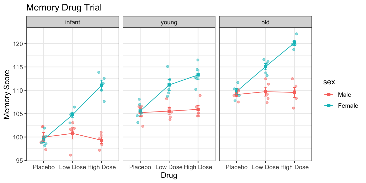
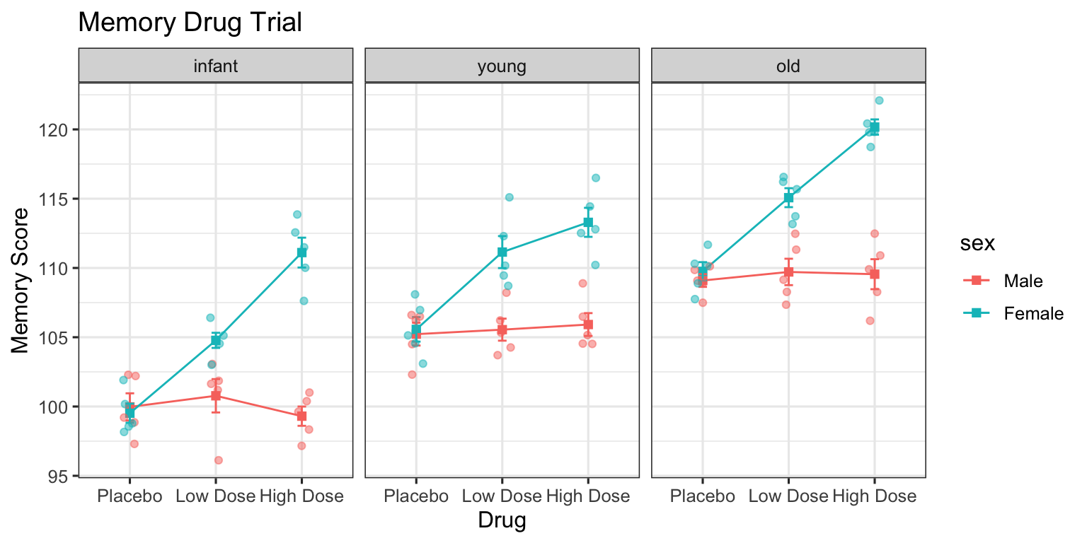
# A tibble: 18 × 6
# Groups:   drug, sex [6]
   drug      sex    age    meanmem    se     n
   <fct>     <fct>  <fct>    <dbl> <dbl> <int>
 1 Placebo   Male   infant   100.  0.982     5
 2 Placebo   Male   young    105.  0.823     5
 3 Placebo   Male   old      109.  0.459     5
 4 Placebo   Female infant    99.5 0.688     5
 5 Placebo   Female young    106.  0.884     5
 6 Placebo   Female old      110.  0.667     5
 7 Low Dose  Male   infant   101.  1.20      5
 8 Low Dose  Male   young    106.  0.795     5
 9 Low Dose  Male   old      110.  0.953     5
10 Low Dose  Female infant   105.  0.546     5
11 Low Dose  Female young    111.  1.16      5
12 Low Dose  Female old      115.  0.684     5
13 High Dose Male   infant    99.3 0.696     5
14 High Dose Male   young    106.  0.824     5
15 High Dose Male   old      110.  1.08      5
16 High Dose Female infant   111.  1.08      5
17 High Dose Female young    113.  1.05      5
18 High Dose Female old      120.  0.551     5

• factor A: Drug: 3 levels (e.g. placebo, low dose, high dose)
• factor B: Sex: 2 levels (e.g. female, male)
• factor C: Age: 3 levels (e.g. infant, young, old)
• DV: memory score (higher is better)
• 3 x 2 x 3 = 18 groups (sometimes called ‘cells’)
• “between subjects” ANOVA: different participants in each group
• 5 participants per group
• 18 x 5 = 90 participants total

3-Way Factorial ANOVA

Code

mem_plot <- ggplot(data=memdata_means,
       mapping = aes(x = drug, 
                     y = meanmem, 
                     color = sex)) + 
  geom_point(pch = 15, 
             size = 2) +
  geom_line(aes(group = sex)) +
  geom_errorbar(aes(ymin = meanmem-se,
                    ymax = meanmem+se), 
                width=.1) +
  geom_jitter(data = memdata,
              mapping = aes(x = drug, y = memory),
              width = 0.1,
              alpha = 0.5) +
  facet_grid(~ age) + 
  labs(title = "Memory Drug Trial",
       x = "Drug",
       y = "Memory Score",
       color = "sex") +
  theme_bw(base_size=12)
mem_plot

3-Way Factorial ANOVA

• 3-way ANOVA tests 7 (!!) omnibus effects:
  • three main effects
  • three 2-way interactions
  • one 3-way interaction

             Df Sum Sq Mean Sq F value   Pr(>F)
drug          2  384.7   192.4  51.148 1.51e-14
sex           1  570.4   570.4 151.656  < 2e-16
age           2 1399.9   699.9 186.113  < 2e-16
drug:sex      2  356.6   178.3  47.404 7.32e-14
drug:age      4    6.6     1.6   0.437    0.781
sex:age       2    4.7     2.3   0.621    0.540
drug:sex:age  4   27.0     6.8   1.795    0.139
Residuals    72  270.8     3.8                 

• is highest order interaction significant?
  • yes: ignore all other effects
  • no: look at set of next highest order interactions

• A x B x C interaction asks “is the 2-way A x B interaction different across levels of C?”
• A x B interactions are averaged over levels of C
• A main effect is averaged over levels of B and C

an example of a 3-way interaction

• the 2-way drug:sex interaction is different across levels of age
• for infants there is no drug:sex interaction
• for young and old there is a two-way drug:sex interaction
  • drug increases memory for females but not for males

3-Way Factorial ANOVA

             Df Sum Sq Mean Sq F value   Pr(>F)
drug          2  384.7   192.4  51.148 1.51e-14
sex           1  570.4   570.4 151.656  < 2e-16
age           2 1399.9   699.9 186.113  < 2e-16
drug:sex      2  356.6   178.3  47.404 7.32e-14
drug:age      4    6.6     1.6   0.437    0.781
sex:age       2    4.7     2.3   0.621    0.540
drug:sex:age  4   27.0     6.8   1.795    0.139
Residuals    72  270.8     3.8                 

• drug:sex:age interaction is not significant
• the drug:sex interaction is significant
• the drug:sex interaction is the same for all levels of age
• age doesn’t appear in any of the interaction terms
• the age main effect is significant

• our Follow-up Plan:
  1. follow up the main effect of age
  2. follow up drug:sex interaction, ignoring age
• (ignore the drug and age main effects)

3-Way Factorial ANOVA

• follow up the main effect of age

library(emmeans)
ageMM <- emmeans(my.anova, specs = ~ age)
pairs(ageMM, adjust="holm")

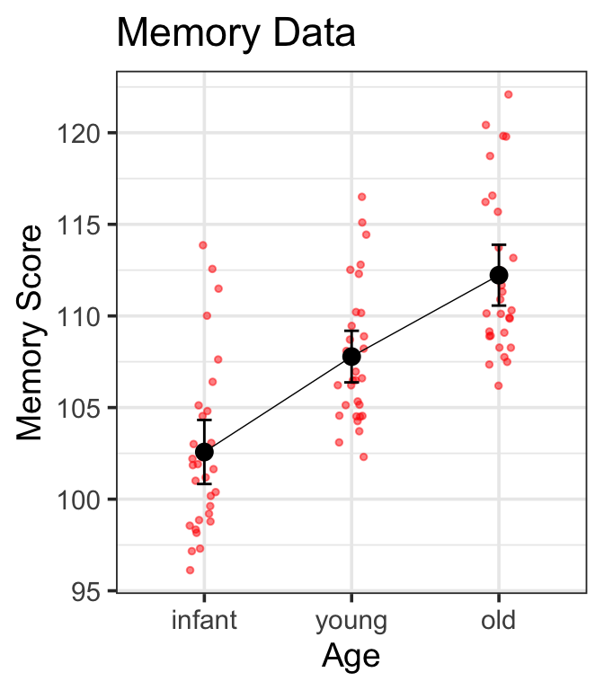
 contrast       estimate    SE df t.ratio p.value
 infant - young    -5.21 0.501 72 -10.399  <.0001
 infant - old      -9.65 0.501 72 -19.273  <.0001
 young - old       -4.44 0.501 72  -8.874  <.0001

Results are averaged over the levels of: drug, sex 
P value adjustment: holm method for 3 tests 

• there is a significant difference in memory score between the infant and young groups, t(72)=-10.4, p<.0001
• there is a significant difference in memory score between the infant and old groups, t(72)=-19.3, p<.0001
• there is a significant difference in memory score between the young and old groups, t(72)=-8.9, p<.0001

 age    emmean    SE df lower.CL upper.CL
 infant    103 0.354 72      102      103
 young     108 0.354 72      107      108
 old       112 0.354 72      112      113

Results are averaged over the levels of: drug, sex 
Confidence level used: 0.95 

Code

set.seed(2812)
memdata %>% 
    group_by(age) %>% 
    summarise(mem = mean(memory),
              sd   = sd(memory),
              N    = n(),
              se   = sd/sqrt(N),
              ci95 = se * qt(.975,N-1)) %>%
    ggplot(aes(x=age,y=mem)) +
        geom_jitter(data=memdata, 
                    aes(x=age,y=memory),
                    width = 0.1,
                    color = "red",
                    alpha = 0.5,
                    size = 1) + 
        geom_errorbar(aes(ymin  = mem-ci95, 
                          ymax  = mem+ci95),
                          width = 0.1) +
        geom_point(aes(x=age,y=mem),
                   size = 3) + 
        geom_line(group=1, aes(x=age,y=mem),
                  color="black", size=.25) +
        labs(x="Age", y="Memory Score",
             title="Memory Data") + 
        theme_bw(base_size=14)

3-Way Factorial ANOVA

• follow up the drug:sex interaction
• simple main effects of drug
• main effect of Drug for “Female” level of sex:

memfemale <- memdata %>% filter(sex=="Female")
female.anova <- aov(memory ~ drug, data=memfemale)
summary(female.anova)

            Df Sum Sq Mean Sq F value   Pr(>F)
drug         2  738.6   369.3   17.51 2.95e-06
Residuals   42  885.7    21.1                 

• main effect of Drug for “Male” level of sex:

memmale <- memdata %>% filter(sex=="Male")
male.anova <- aov(memory ~ drug, data=memmale)
summary(male.anova)

            Df Sum Sq Mean Sq F value Pr(>F)
drug         2    2.7   1.356   0.069  0.933
Residuals   42  823.2  19.600               

• so let’s follow up the main effect of drug in Females, with pairwise posthoc tests

Code

set.seed(2812)
memdata %>% 
    group_by(drug,sex) %>% 
    summarise(mem = mean(memory),
              sd   = sd(memory),
              N    = n(),
              se   = sd/sqrt(N),
              ci95 = se * qt(.975,N-1)) %>%
    ggplot(aes(x=drug,y=mem)) +
        geom_jitter(data=memdata, 
                    aes(x=drug,y=memory, color=sex),
                    width = 0.1,
                    color = "red",
                    alpha = 0.5,
                    size = 1) + 
        geom_errorbar(aes(ymin  = mem-ci95, 
                          ymax  = mem+ci95),
                          width = 0.1) +
        geom_point(aes(x=drug,y=mem),
                   size = 3) + 
        geom_line(group=1, aes(x=drug,y=mem),
                  color="black", size=.25) +
        facet_grid(~ sex) + 
        labs(x="Drug", y="Memory Score",
             title="Memory Data") + 
        theme_bw(base_size=14)

• we just did one one-way ANOVA using the subset of data for Females and another using the subset of data for Males

3-Way Factorial ANOVA

• follow up the drug:sex interaction
• pairwise posthoc tests of the main effect of drug in Females
• using the female.anova object (which was made using only data for Females)

drugMfemale <- emmeans(female.anova, specs = ~ drug)
pairs(drugMfemale, adjust="holm")

 contrast             estimate   SE df t.ratio p.value
 Placebo - Low Dose      -5.38 1.68 42  -3.211  0.0051
 Placebo - High Dose     -9.91 1.68 42  -5.911  <.0001
 Low Dose - High Dose    -4.53 1.68 42  -2.699  0.0100

P value adjustment: holm method for 3 tests 

3-Way Factorial ANOVA

• follow up the drug:sex interaction
• pairwise posthoc tests of the main effect of drug in Females
• using emmeans with the my.anova 3-way ANOVA gives us a more powerful test because it uses the error term from the 3-factor ANOVA

emmeans(my.anova, specs = ~drug:sex) %>% 
  pairs(simple="drug", adjust="holm")

sex = Male:
 contrast             estimate    SE df t.ratio p.value
 Placebo - Low Dose     -0.582 0.708 72  -0.822  1.0000
 Placebo - High Dose    -0.160 0.708 72  -0.227  1.0000
 Low Dose - High Dose    0.422 0.708 72   0.595  1.0000

sex = Female:
 contrast             estimate    SE df t.ratio p.value
 Placebo - Low Dose     -5.385 0.708 72  -7.604  <.0001
 Placebo - High Dose    -9.911 0.708 72 -13.996  <.0001
 Low Dose - High Dose   -4.527 0.708 72  -6.392  <.0001

Results are averaged over the levels of: age 
P value adjustment: holm method for 3 tests 

• Like when we did simple main effects in our 2x2 design earlier, and we computed a custom F-test using the error term from the full ANOVA