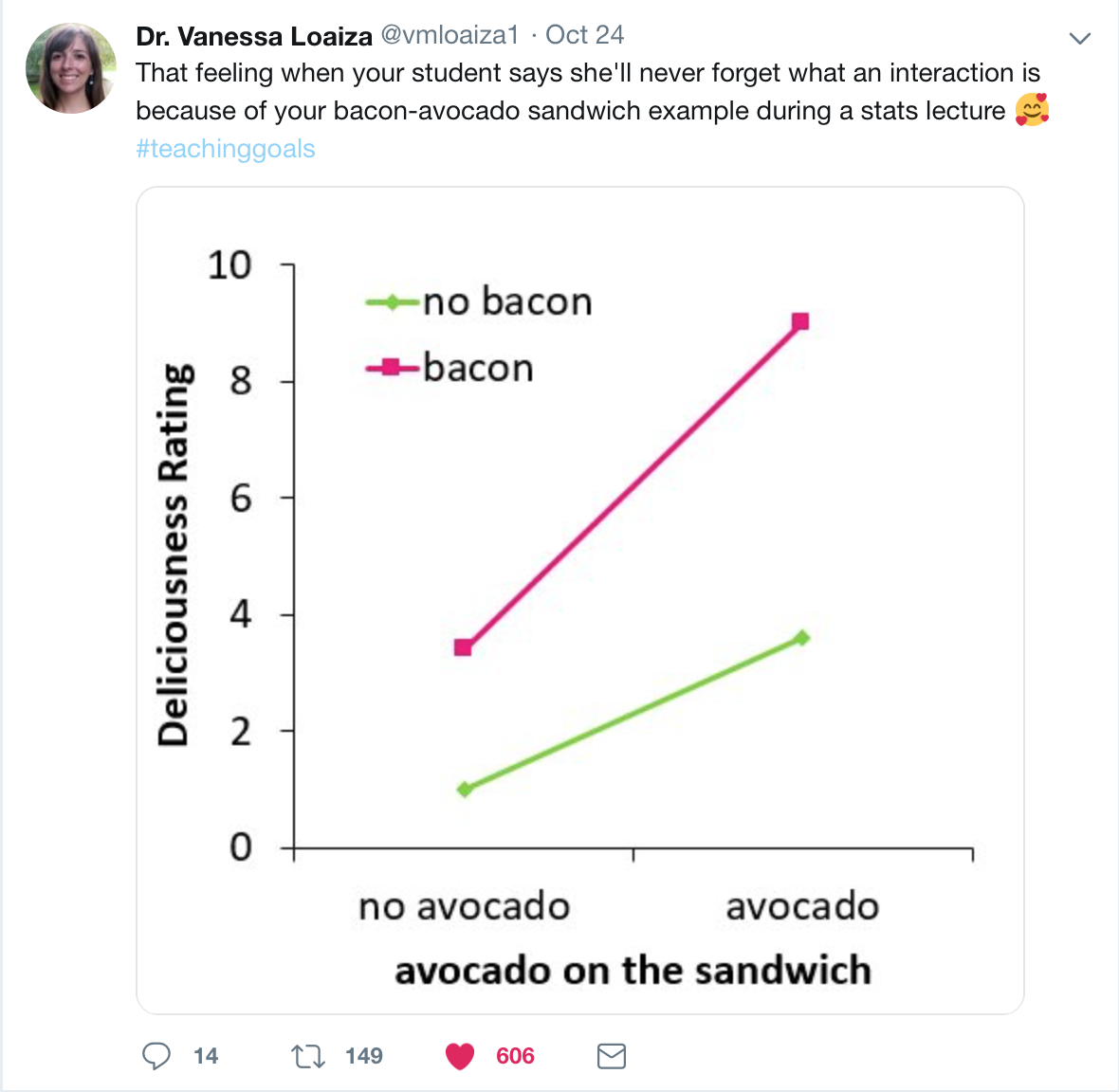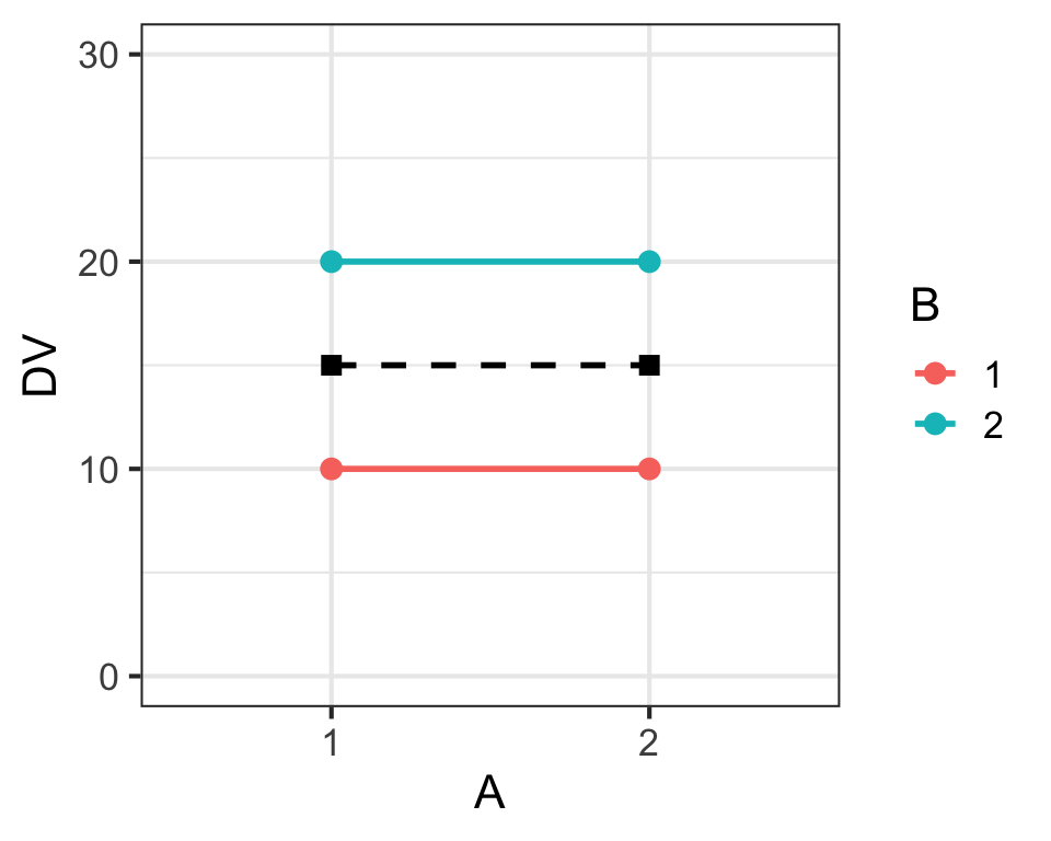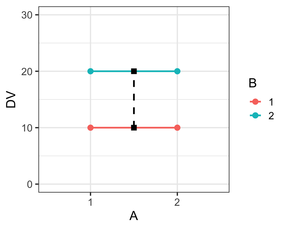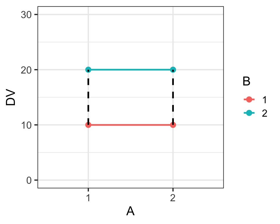
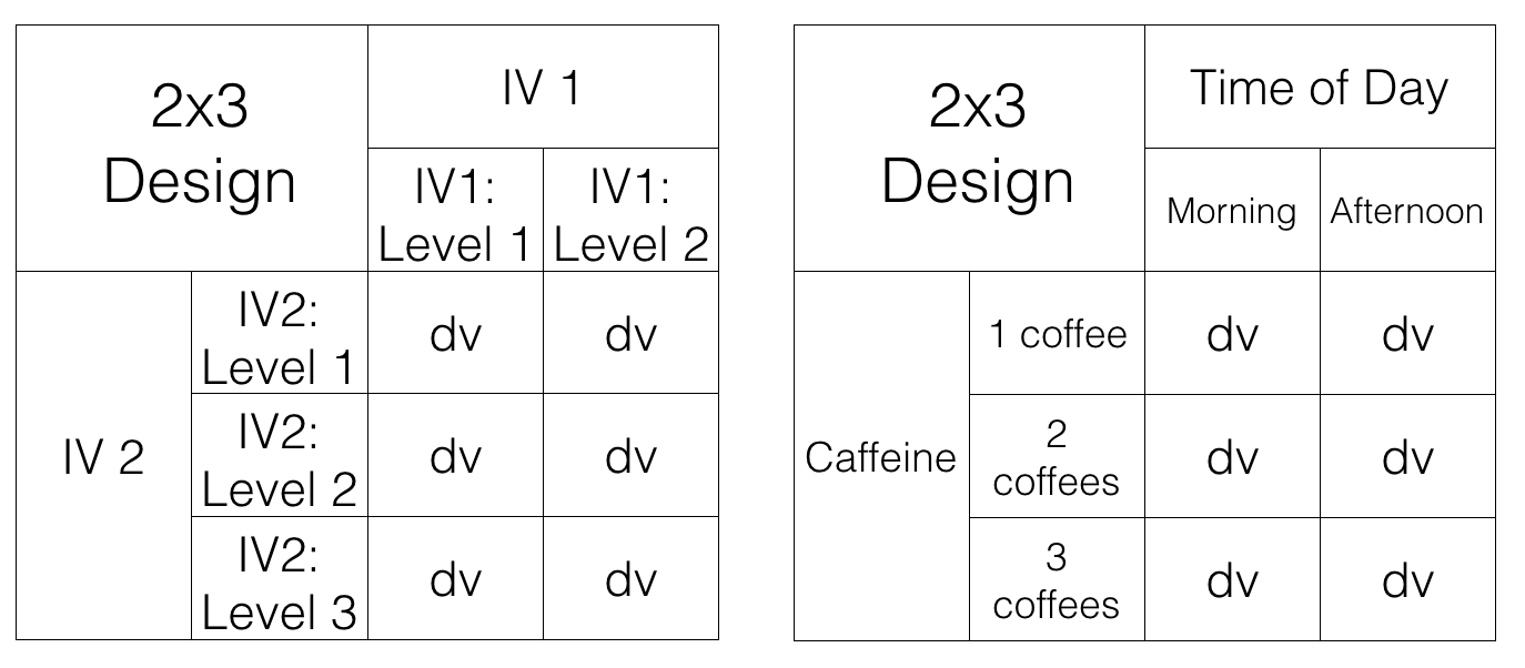

Main Effects & Interaction
- SSdrug + SSres = SStot
- 3.453 + 1.392 = 4.85
            Df Sum Sq Mean Sq F value   Pr(>F)
drug         2  3.453  1.7267   18.61 8.65e-05
Residuals 15 1.392 0.0928 - SStherapy + SSres = SStot
- 0.467 + 4.378 = 4.85
            Df Sum Sq Mean Sq F value Pr(>F)
therapy      1  0.467  0.4672   1.708   0.21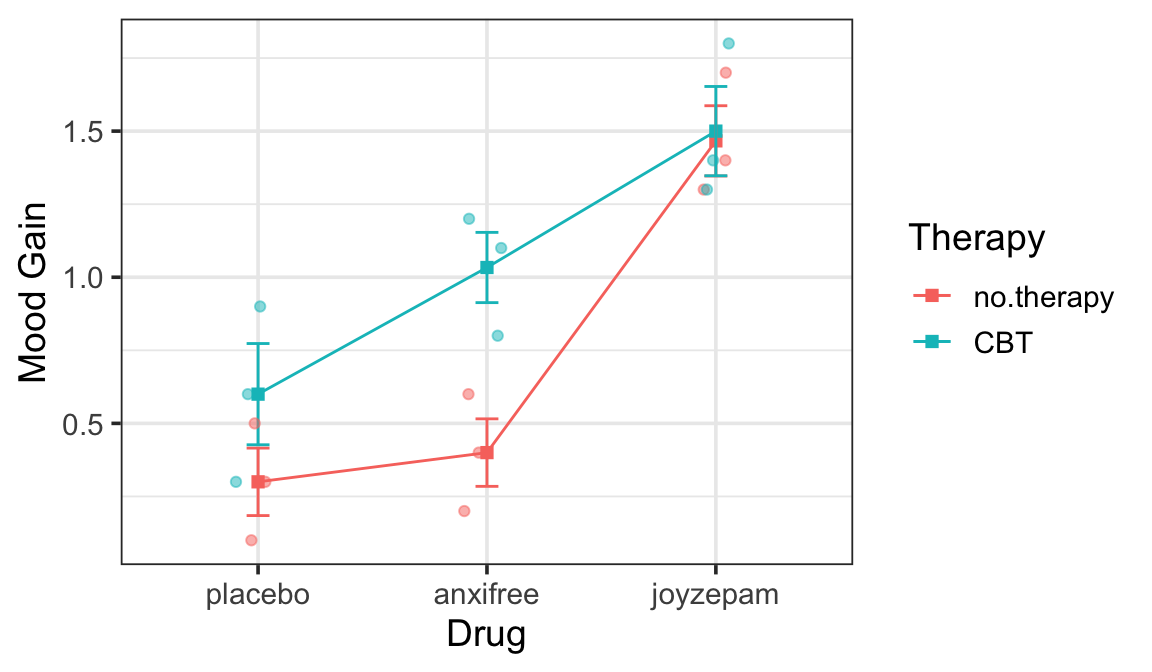
Residuals 16 4.378 0.2736 - SSdrug + SStherapy + SSres = SStot
- 3.453 + 0.467 + 0.924 = 4.85
            Df Sum Sq Mean Sq F value   Pr(>F)
drug         2  3.453  1.7267  26.149 1.87e-05
therapy      1  0.467  0.4672   7.076   0.0187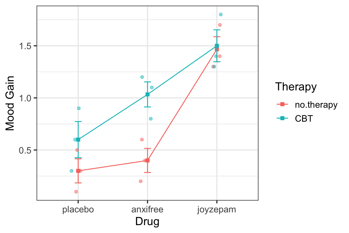
Residuals 14 0.924 0.0660 - SSdrug + SStherapy + SSinteraction + SSres = SStot
- 3.453 + 0.467 + 0.271 + 0.653 = 4.85
             Df Sum Sq Mean Sq F value   Pr(>F)
drug          2  3.453  1.7267  31.714 1.62e-05
therapy       1  0.467  0.4672   8.582   0.0126
drug:therapy  2  0.271  0.1356   2.490   0.1246
Residuals 12 0.653 0.0544 - SSres is even smaller!
- reduces unexplained variance in the DV
- denominator of F-statistic is smaller
- F-statistics for our main effects are bigger
- p-values for our main effects are smaller