Oneway ANOVA: follow-up tests & statistical power
Week 8
Last week
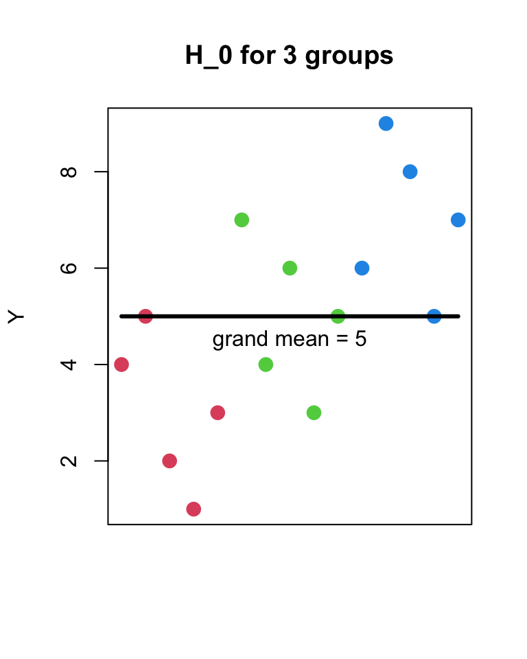
- H_{0}
- Y_{ij} = \mu + \epsilon_{ij}
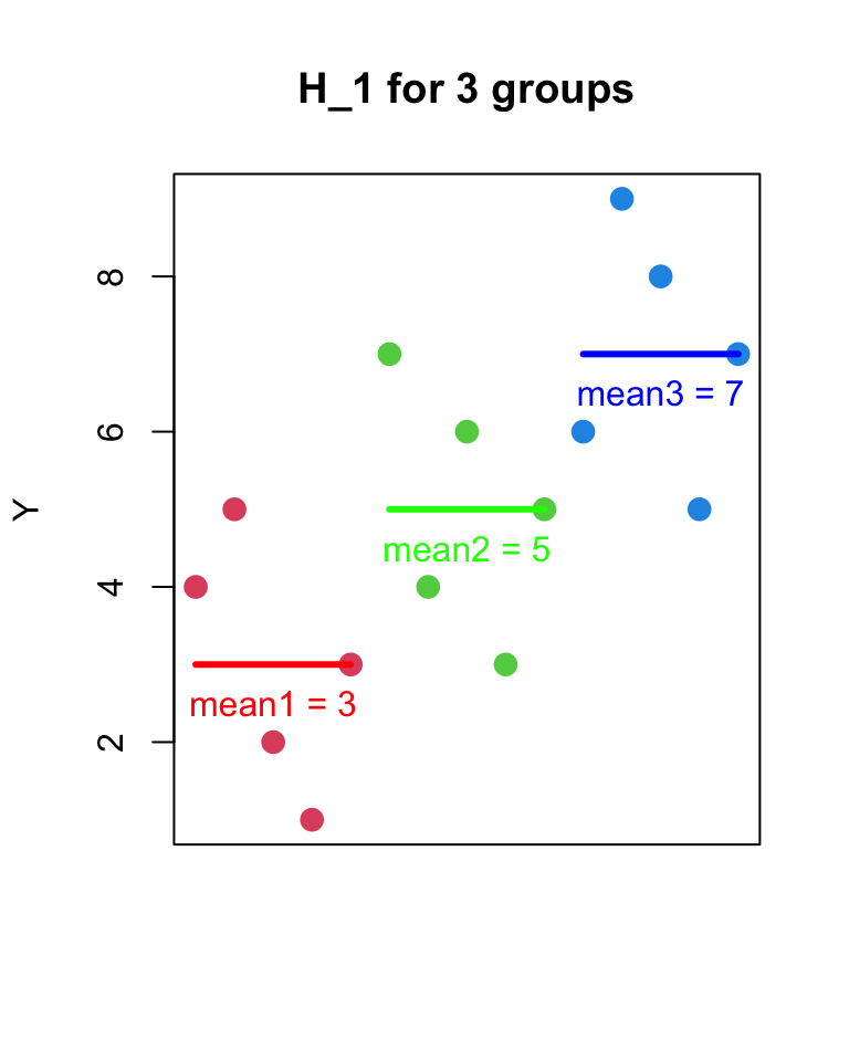
- H_{1}
- Y_{ij} = \mu_{j} + \epsilon_{ij}
Statistical Significance vs Effect Size

ANOVA: Omnibus F-test

- which means are different?
- we can conduct “post-hoc” tests
- like a series of pairwise t-tests
- (with some slight changes)
ANOVA: Follow-up tests
ANOVA: Follow-up tests: pairwise.t.test()
pairwise.t.test()is a function in base R- feed it your DV and your IV
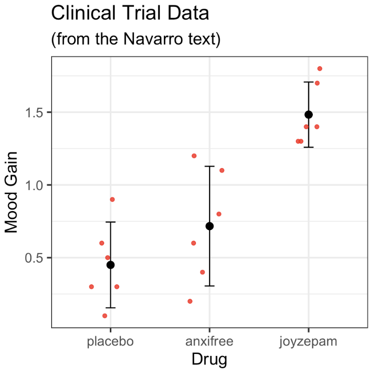
pairwise.t.test( x = clin.trial$mood.gain,
                 g = clin.trial$drug,
                 p.adjust.method = "none") # we will change this later
    Pairwise comparisons using t tests with pooled SD

data:  clin.trial$mood.gain and clin.trial$drug

         placebo anxifree
anxifree 0.15021 -
joyzepam 3e-05   0.00056

P value adjustment method: none
ANOVA: Follow-up tests: posthocPairwiseT()
posthocPairwiseT()is a function from thelsrpackage- feed it your anova model object
review: Type-I Errors
- a Type-I error is when you reject the null hypothesis when it is actually true
- you conclude there is a difference when there is actually no difference

Type-I Error rate: simulations
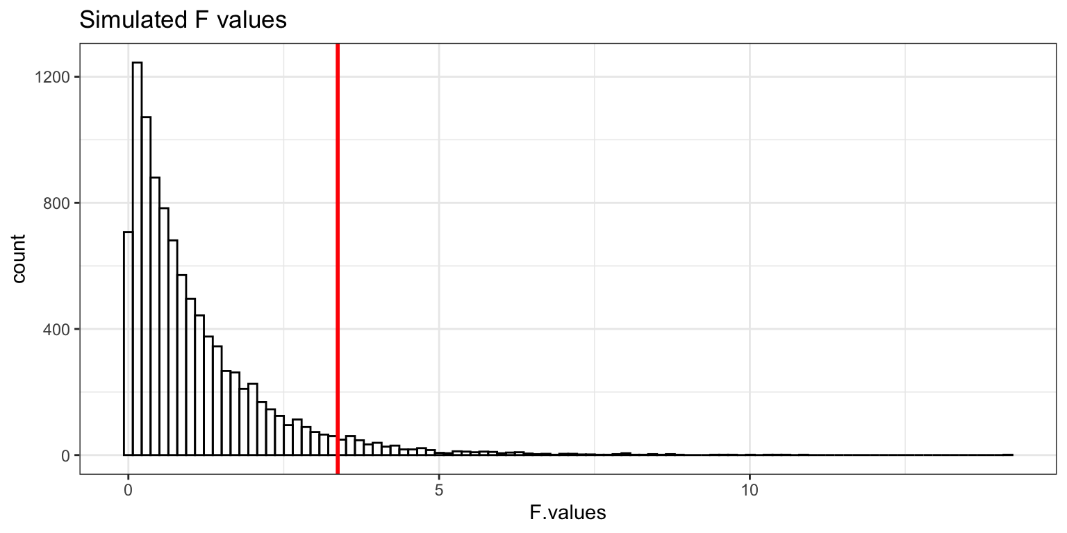
Type-I Error rate: simulations
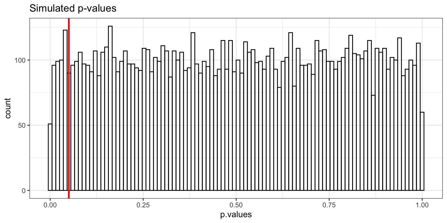
Type-I Error rate
- H_{0} is actually true: then \alpha determines our Type-I error rate
- H_{0} is actually false: rejecting H_{0} is the correct decision; no Type-I error
Type-II Error rate
- a Type-II error is when you fail to reject the null hypothesis even though it is actually false—the alternate hypothesis is true
- you conclude there is not a difference when there is actually is one

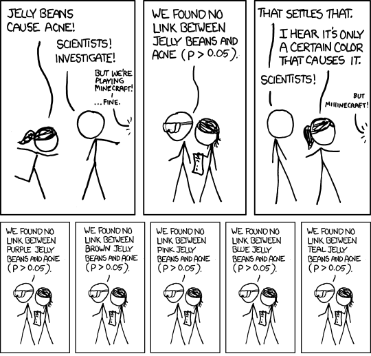
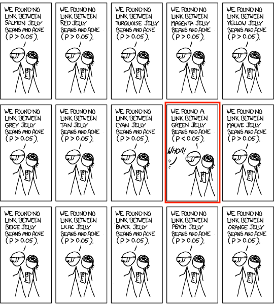
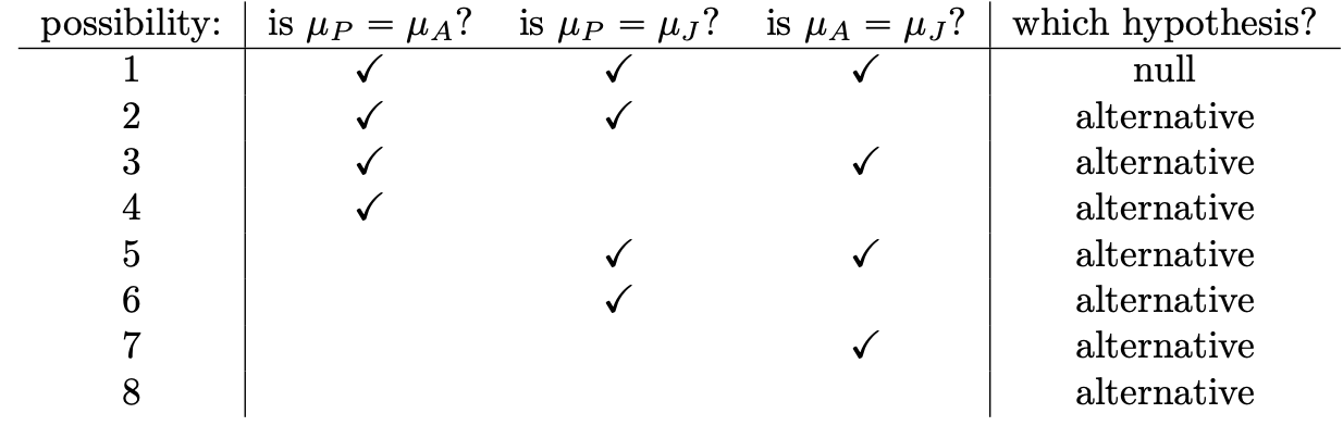
Multiple Comparisons
- how many possible pairwise tests?
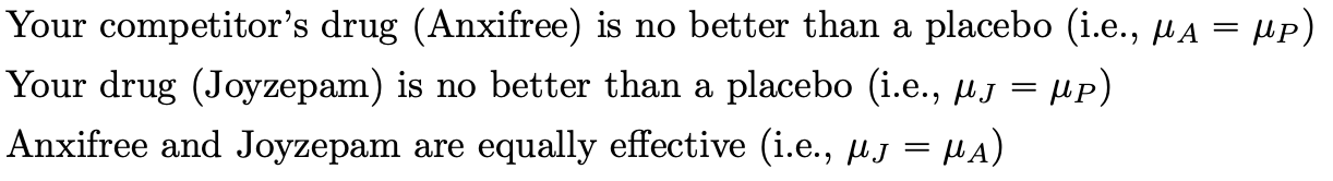
- placebo vs anxifree
- placebo vs joyzepam
- anxifree vs joyzepam
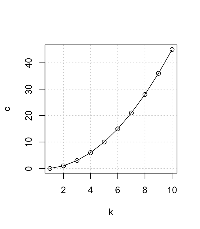
- For K groups the number of possible pairwise tests is:
- K(K-1)/2
Multiple Comparisons
- For K groups the number of possible pairwise tests is:
- K(K-1)/2
- for 3 groups: 3*(3-1)/2 = 3
- for 4 groups: 4*(4-1)/2 = 6
- for 6 groups: 6*(6-1)/2 = 15
- for 10 groups: 10*(10-1)/2 = 45 !
Multiple Comparisons
- 3 post-hoc tests:
- placebo vs anxifree
- placebo vs joyzepam
- anxifree vs joyzepam
- each test has a p-value
- we make a decision about each test based on \alpha = .05
- Q: is our overal (family-wise) Type-I error rate still 5 %?
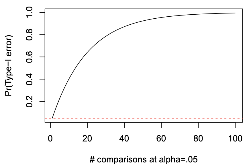
Multiple Comparisons
- is family-wise Type-I error still 5 %?
- Answer: No!
- Type-I error rate is inflated
- Type-I error rate on the whole family of tests is way above 5 %
- Pr(Type-I error) = 1 - (1 - \alpha)^{C}
- C is the number of post-hoc tests
Multiple Comparisons
- Pr(Type-I error) = 1 - (1 - \alpha)^{C}
- when C=3
- we get 14.3% family-wise Type-I error rate
Multiple Comparisons
- Pr(Type-I error) = 1 - (1 - \alpha)^{C}
Multiple Comparisons
- Pr(Type-I error) = 1 - (1 - \alpha)^{C}

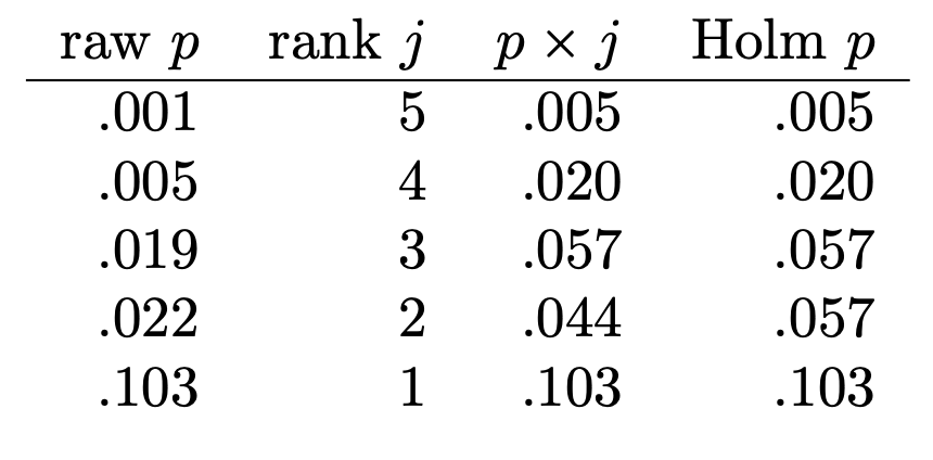
Bonferroni-Holm Correction
- corrects more for most significant tests and less for less significant tests