Multiple Regression II
Week 6
Final Exam

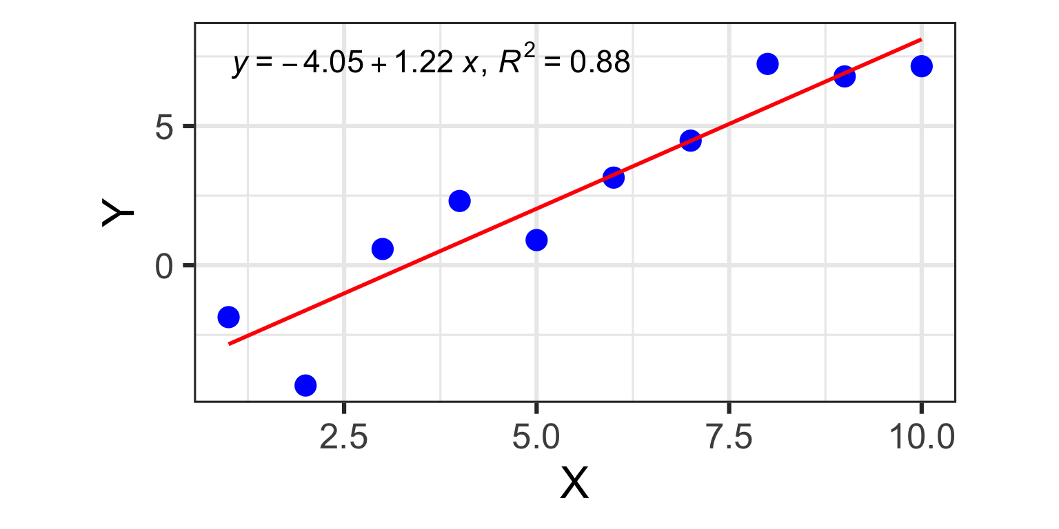
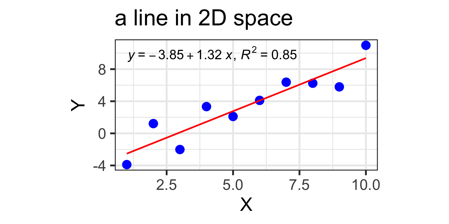
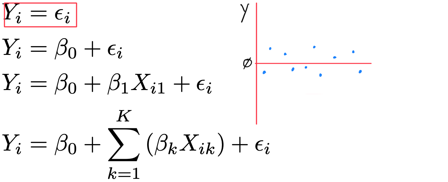
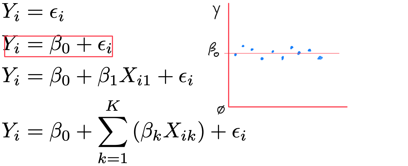
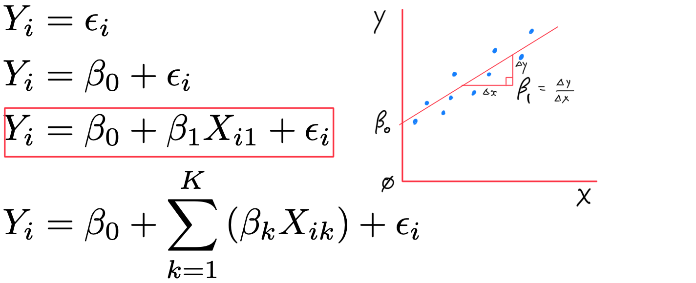
1 predictor: a line in 2D
- Y_{i} = \beta_{0} + \beta_{1} X + \varepsilon_{i}
- one dependent variable Y (the variable to be predicted)
- one independent variable X (the variable we are using to predict Y)
- N different observations of each (X_{i},Y_{i}), for i=1 \dots N
- two model coefficients, \beta_{0} (intercept) & \beta_{1} (slope)
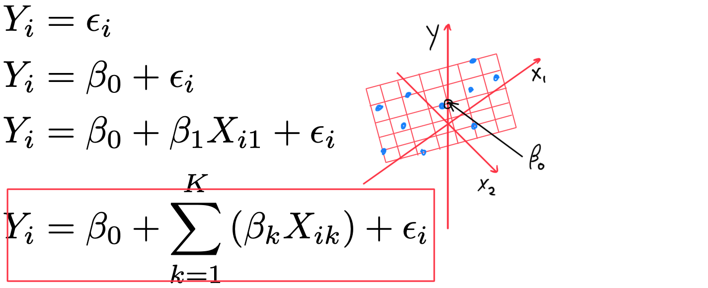
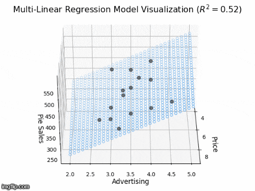
2 predictors: a 2D plane in 3D
- Y_{i} = \beta_{0} + \beta_{1} X_{i1} + \beta_{2} X_{i2} +\varepsilon_{i}
- Y: “Pie Sales”
- X_{1}: “Price”, X_{2} is “Advertising”
- \beta_{1}: dependence of Pie Sales (Y) on Price (X_{1})
- \beta_{2}: dependence of Pie Sales (Y) on Advertising (X_{2})
- \beta_{0}: predicted Pie Sales (Y) when Price and Advertising are both zero
- a 2D plane in 3D space
![]()
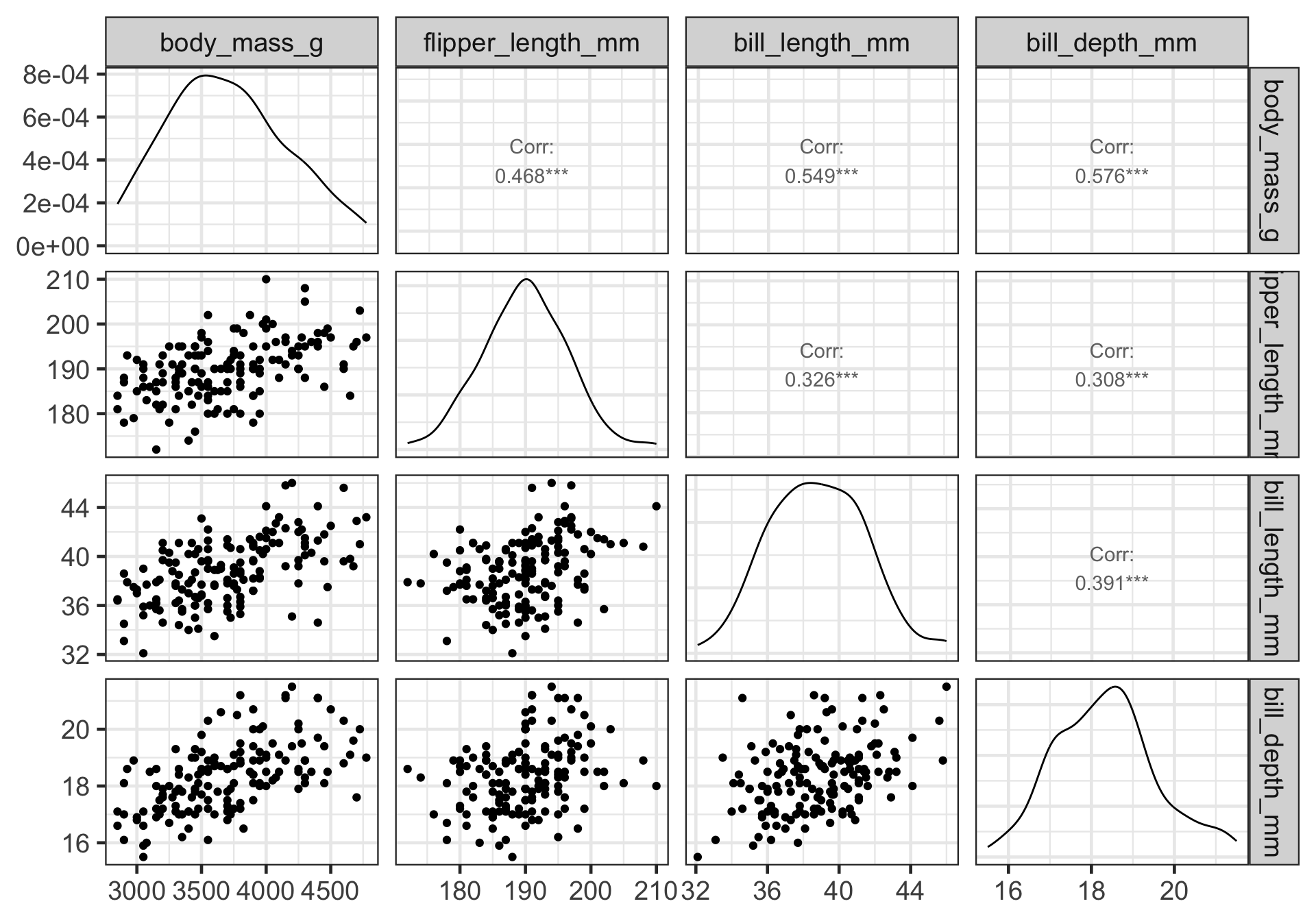
An Example: palmerpenguins

The penguins data from the palmerpenguins package contains size measurements for 344 penguins from three species observed on three islands in the Palmer Archipelago, Antarctica.
2. Look at correlation matrix
4. Check assumptions
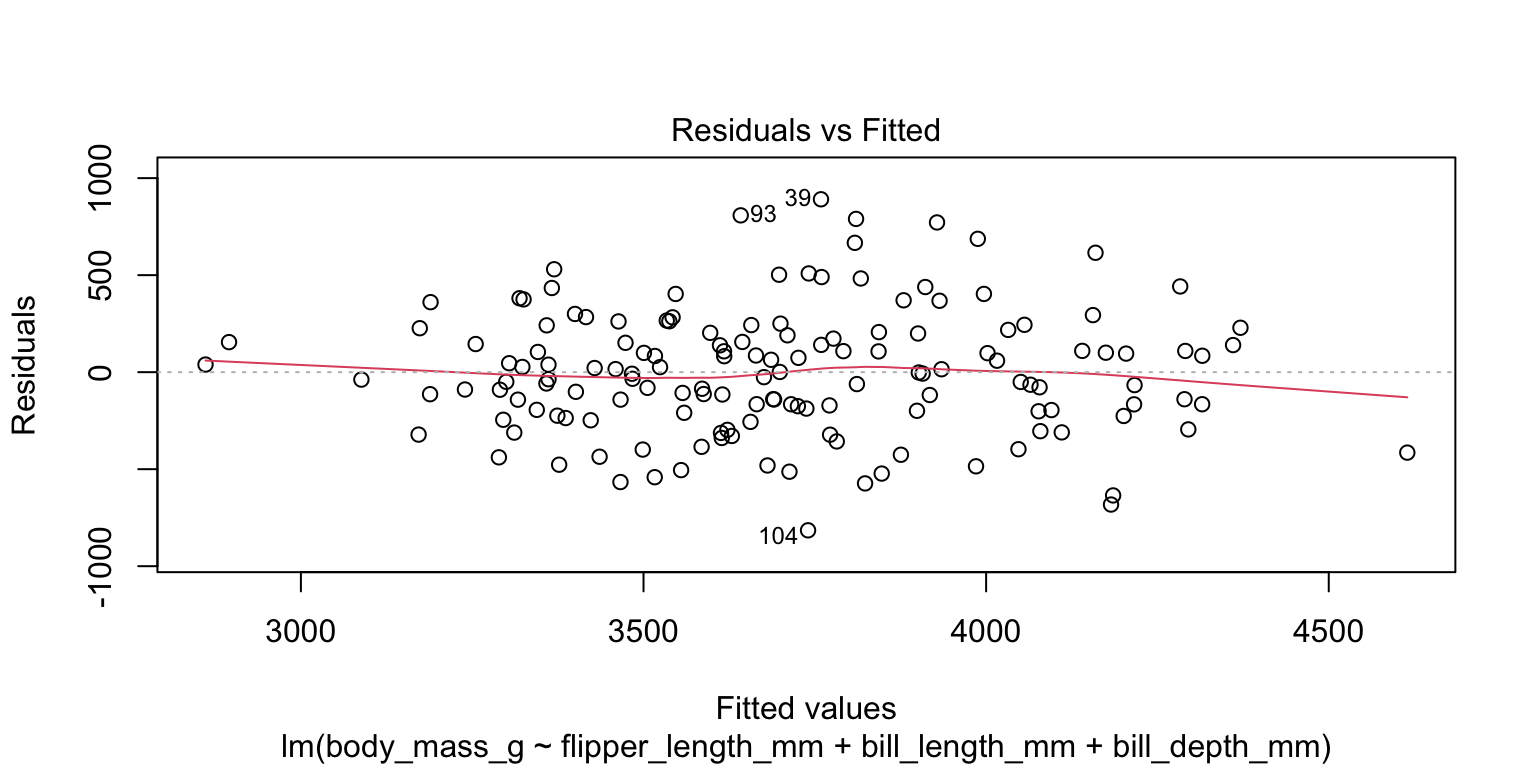
- check the linearity assumption
- plot the fitted values against the residuals—no obvious indication of non-linearity
4. Check assumptions
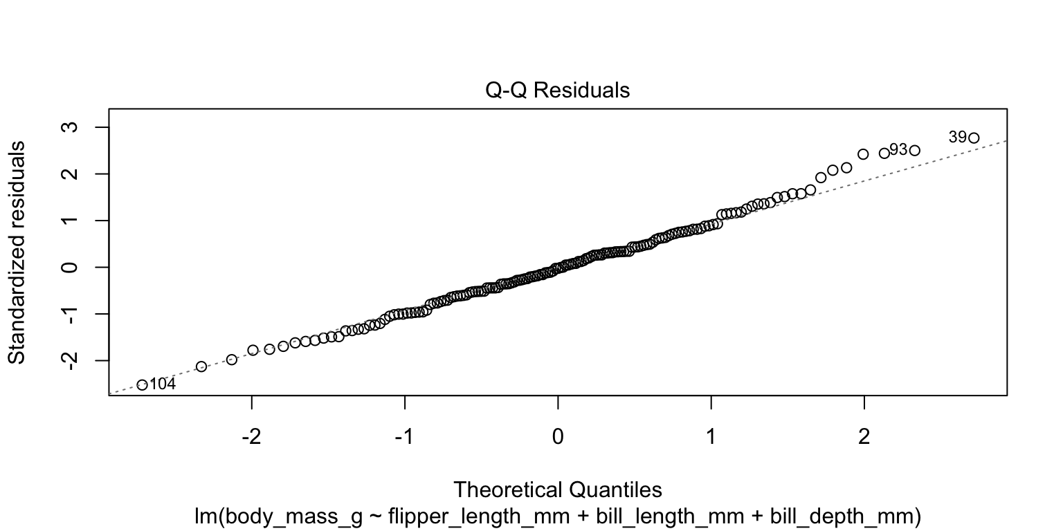
- check the normality assumption
- produce a Q-Q plot—no obvious indication of non-linearity
4. Check assumptions
- check the homoscedasticity assumption
- look at plot of residuals—no sign of variance change across range

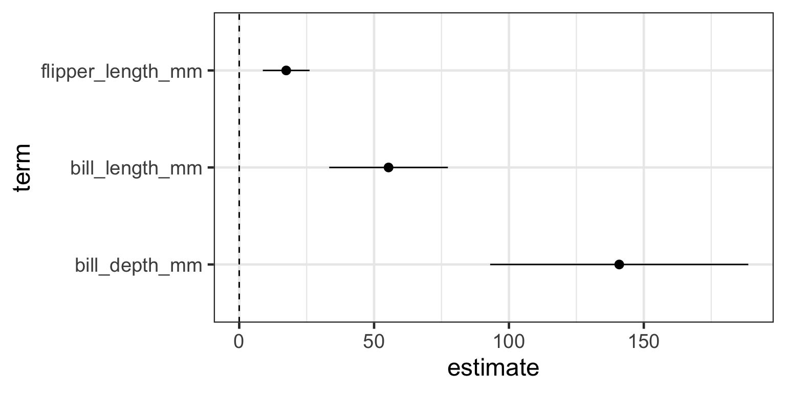
5. Interpret the model
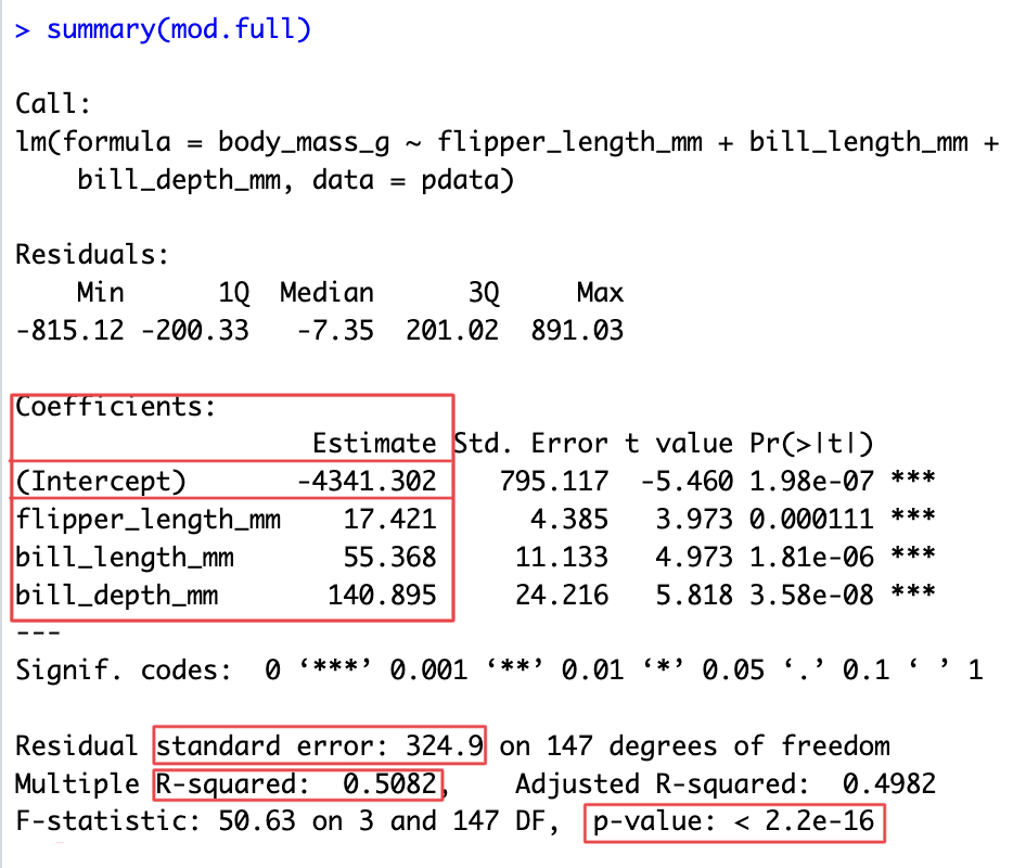
5. Interpret the model
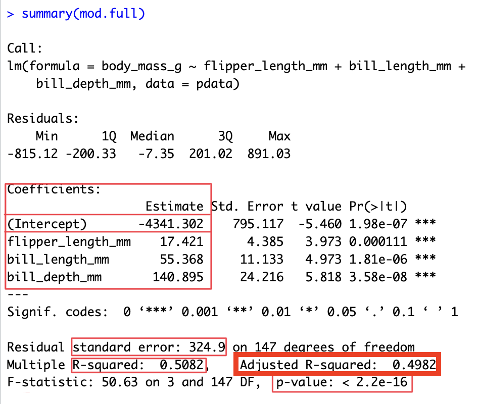
5. Interpret the model
# A tibble: 3 × 7
  term              estimate std.error statistic      p.value conf.low conf.high
  <chr>                <dbl>     <dbl>     <dbl>        <dbl>    <dbl>     <dbl>
1 flipper_length_mm     17.4      4.39      3.97 0.000111         8.76      26.1
2 bill_length_mm        55.4     11.1       4.97 0.00000181      33.4       77.4
3 bill_depth_mm 141. 24.2 5.82 0.0000000358 93.0 189. - plot model coefficients (slopes) relative to zero
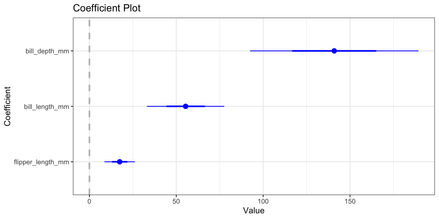
5. Interpet the model
- OR: You can use the
coefplotpackage to more easily plot coefficients and their confidence intervals - just pass it your
lm()model object
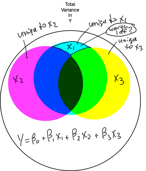
6. Refine the model: unique variance
6. Refine the model: unique variance
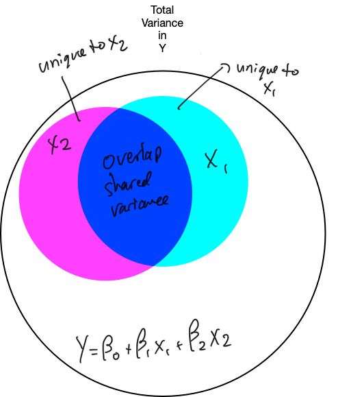
6. Refine the model: unique variance
6. Refine the model
- recall the significance test of the model “as a whole”:
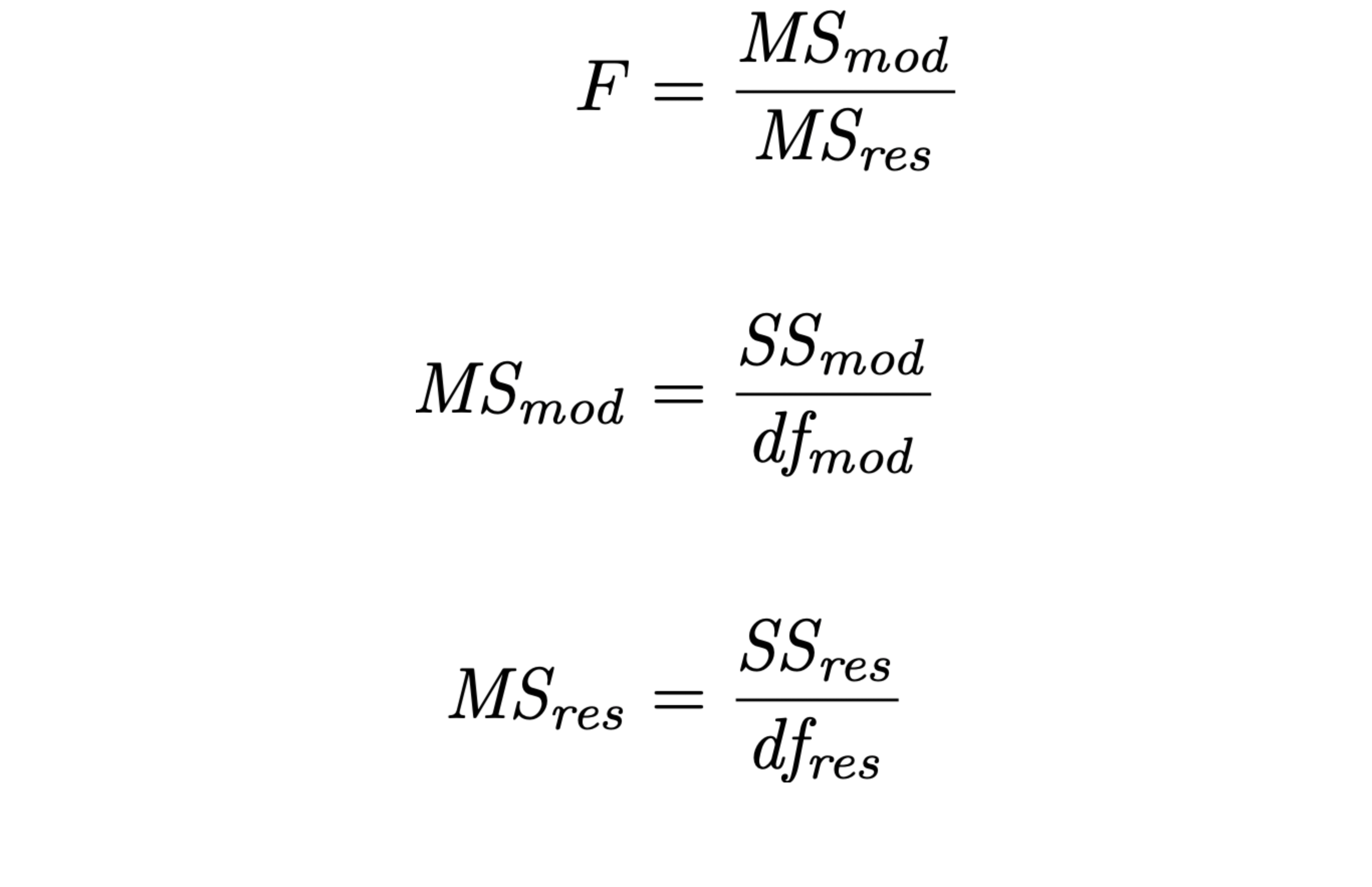
6. Refine the model
- recall the significance test of the model “as a whole”:
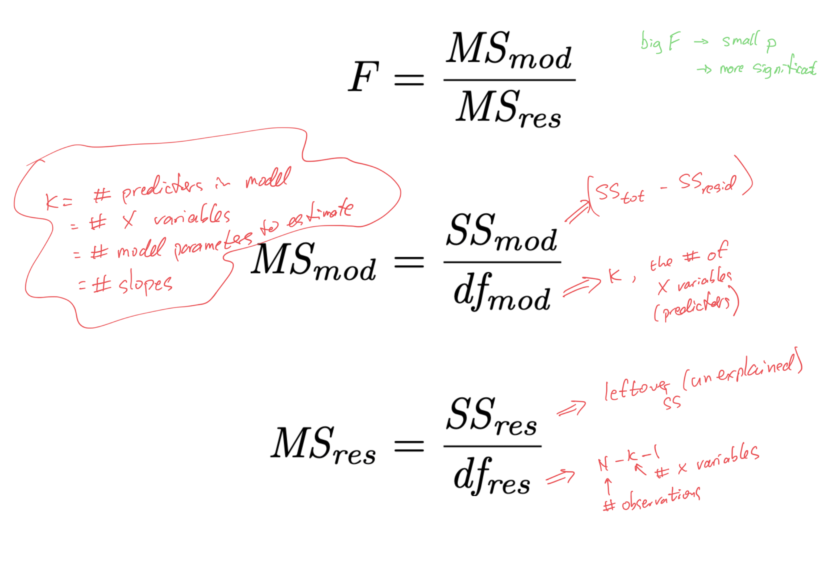
6. Refine the model
- recall the significance test of the model “as a whole”:
6. Refine the model
- recall the significance test of the model “as a whole”:
6. Refine the model
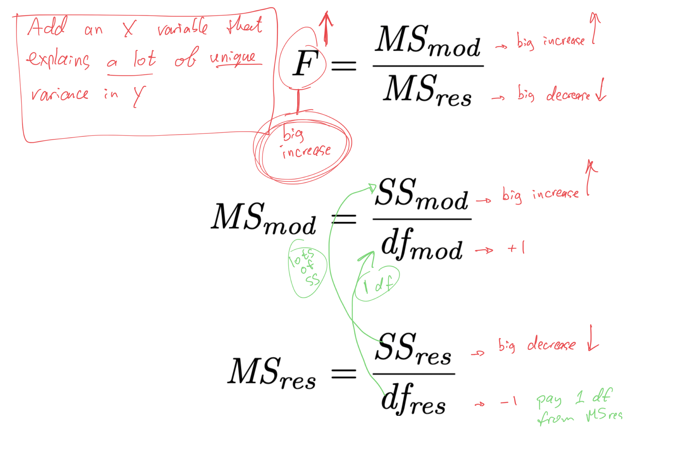
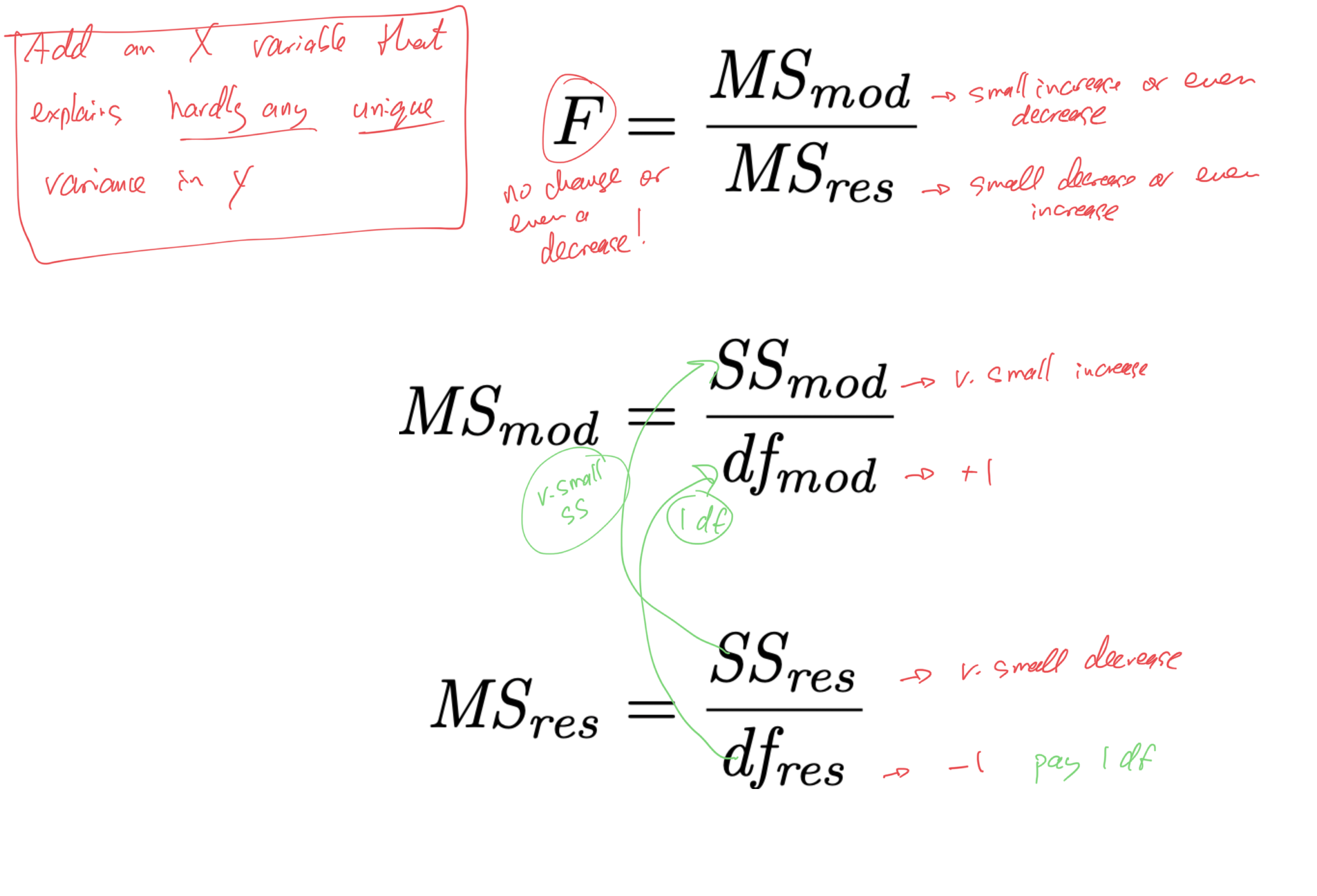
- when we add an X variable to the model,
- we “pay” by taking 1 df out of MSres
- smaller MSres denominator means larger MSres
- larger MSres means smaller F
- smaller F means larger p
- larger p means less significant
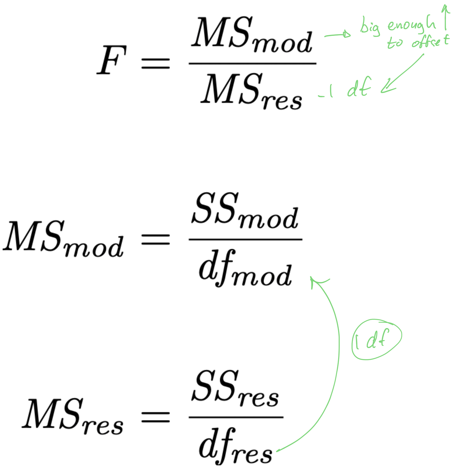
- if we are to “pay” 1 df from the MSres denominator, to make it worth it,
- the X variable should explain a lot of unique variance in Y
- it should increase SSmod and decrease SSres enough to offset the increase in MSres caused by the removal of 1 df
6. Refine the model
- if we are to “pay” 1 df from the MSres denominator, to make it worth it,
- the X variable should explain enough unique variance in Y
- it should increase SSmod and decrease SSres enough to offset the change in MSres caused by the removal of 1 df
- how much is “enough”?
- how much unique variance does an X variable need to explain in order to offset having to “pay” with 1 df from the error term (from MSres)?
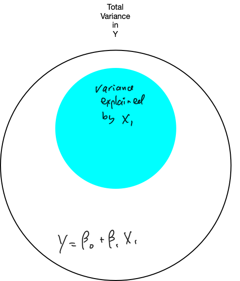
6. Refine the model: Adj. R^{2}
R^{2} = 1 - \frac{\mathit{SS_{res}}}{\mathit{SS_{tot}}} \text{adj.}R^{2} = 1 - \left( \frac{\mathit{SS_{res}}}{\mathit{SS_{tot}}} \times \frac{N-1}{N-K-1} \right)
- adding predictors to model will always increase R^{2}
- takes into account the number of parameters (X variables) K
- adj. R^{2} will only increase if the new X variable improves the model performance more than what you’d expect by chance
6. Refine the model: unique variance
6. Refine the model: unique variance
6. Refine the model: unique variance
Linear Models
Linear Models
Linear Models
Linear Models