Linear Regression II & Intro to Multiple Regression

Week 5

scatterplot plus regression line

R: intercept and slope

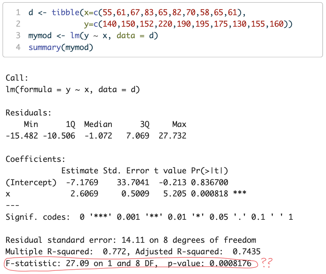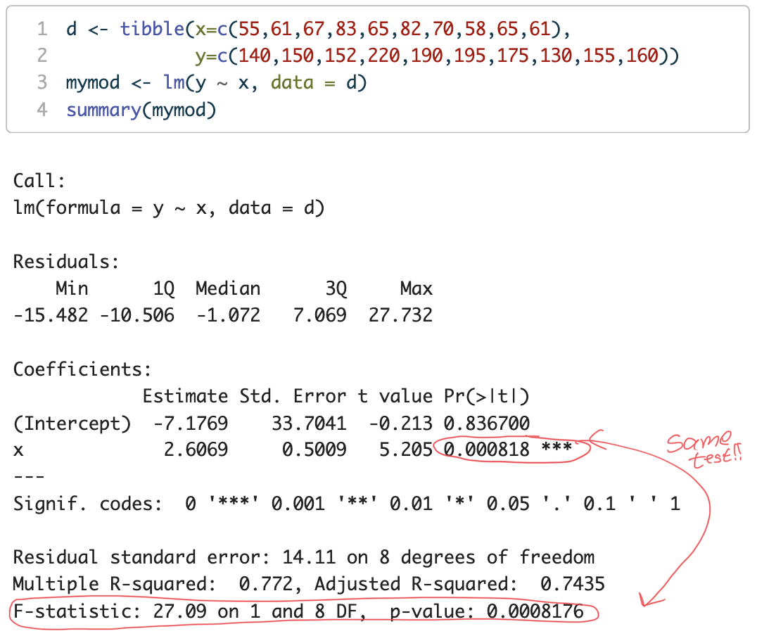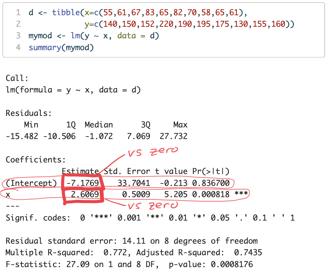
library(tidyverse)
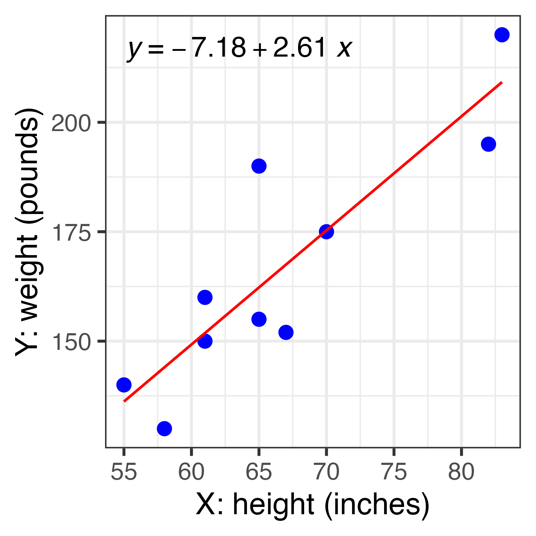
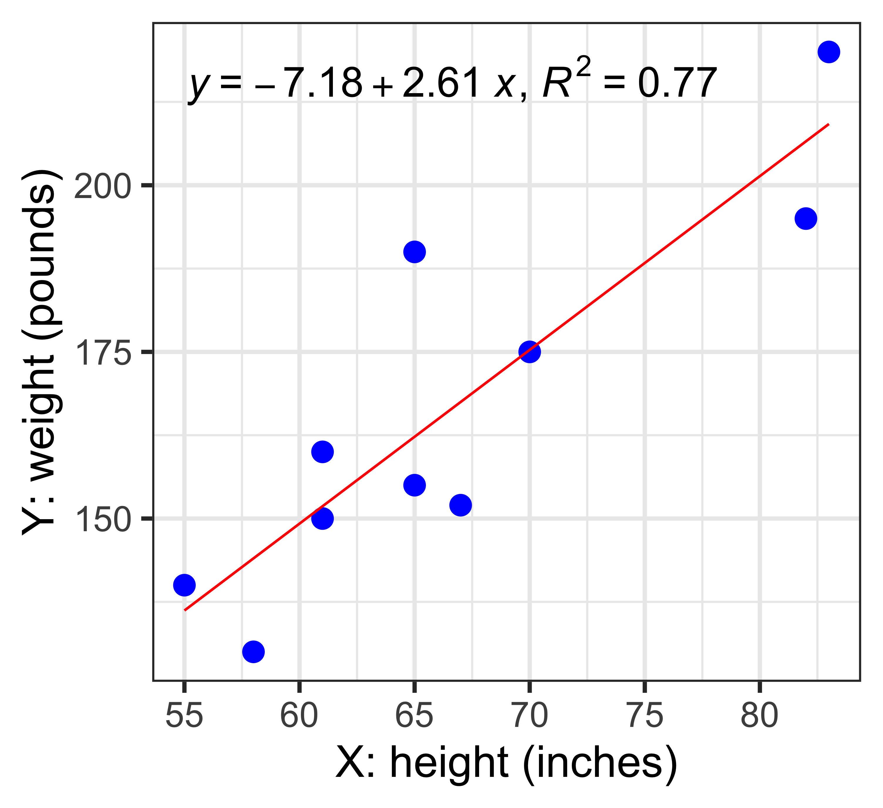
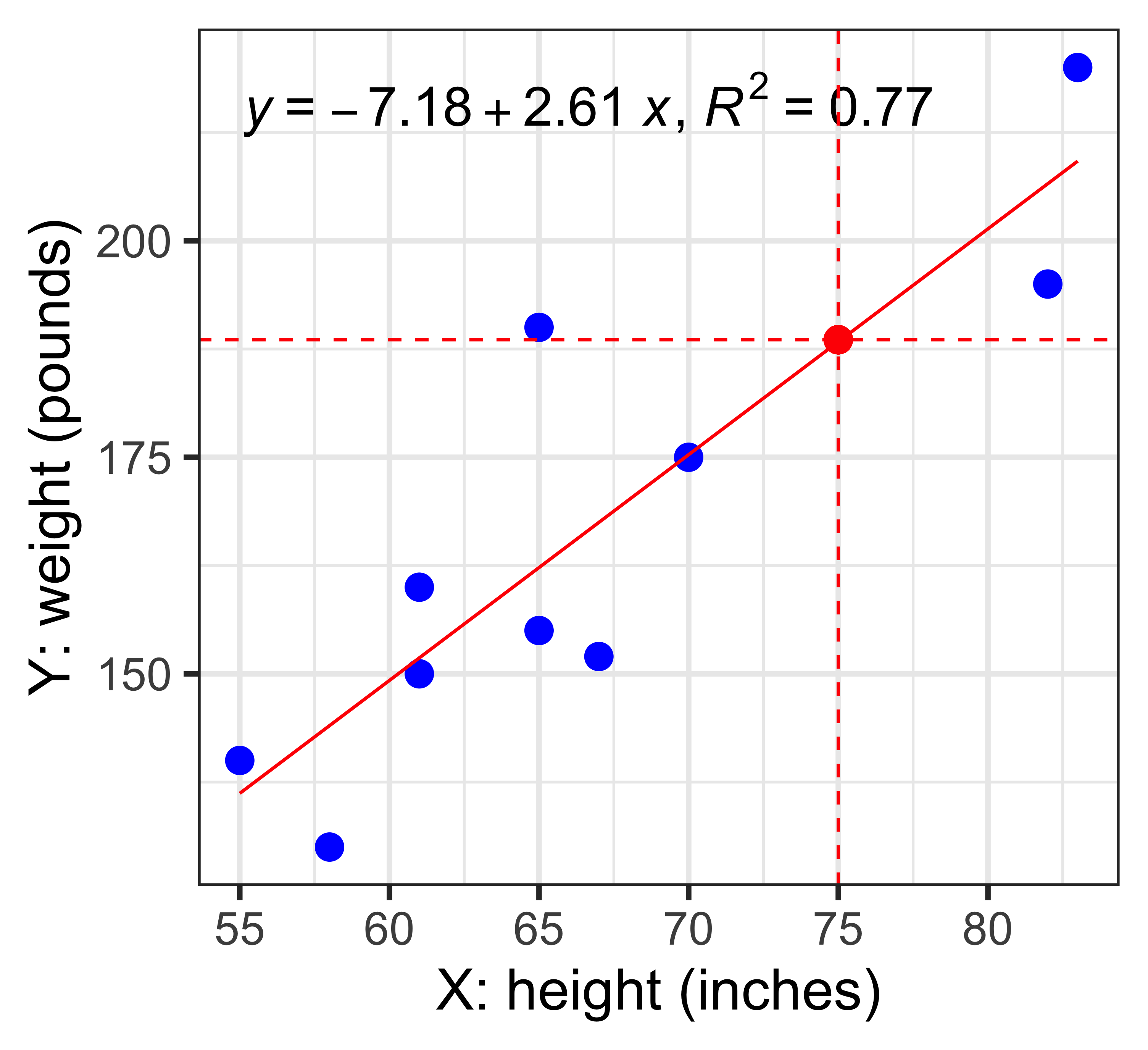
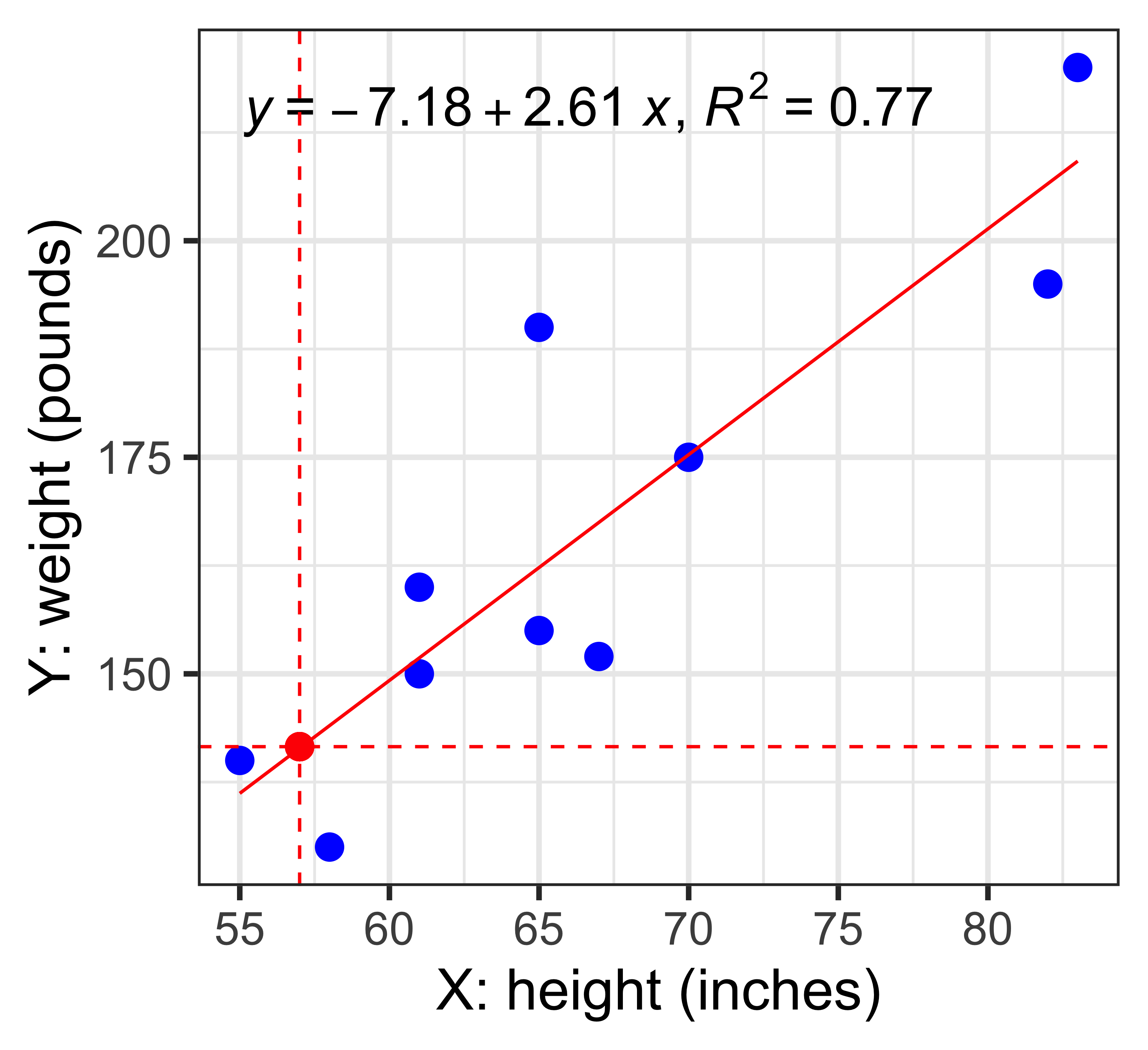
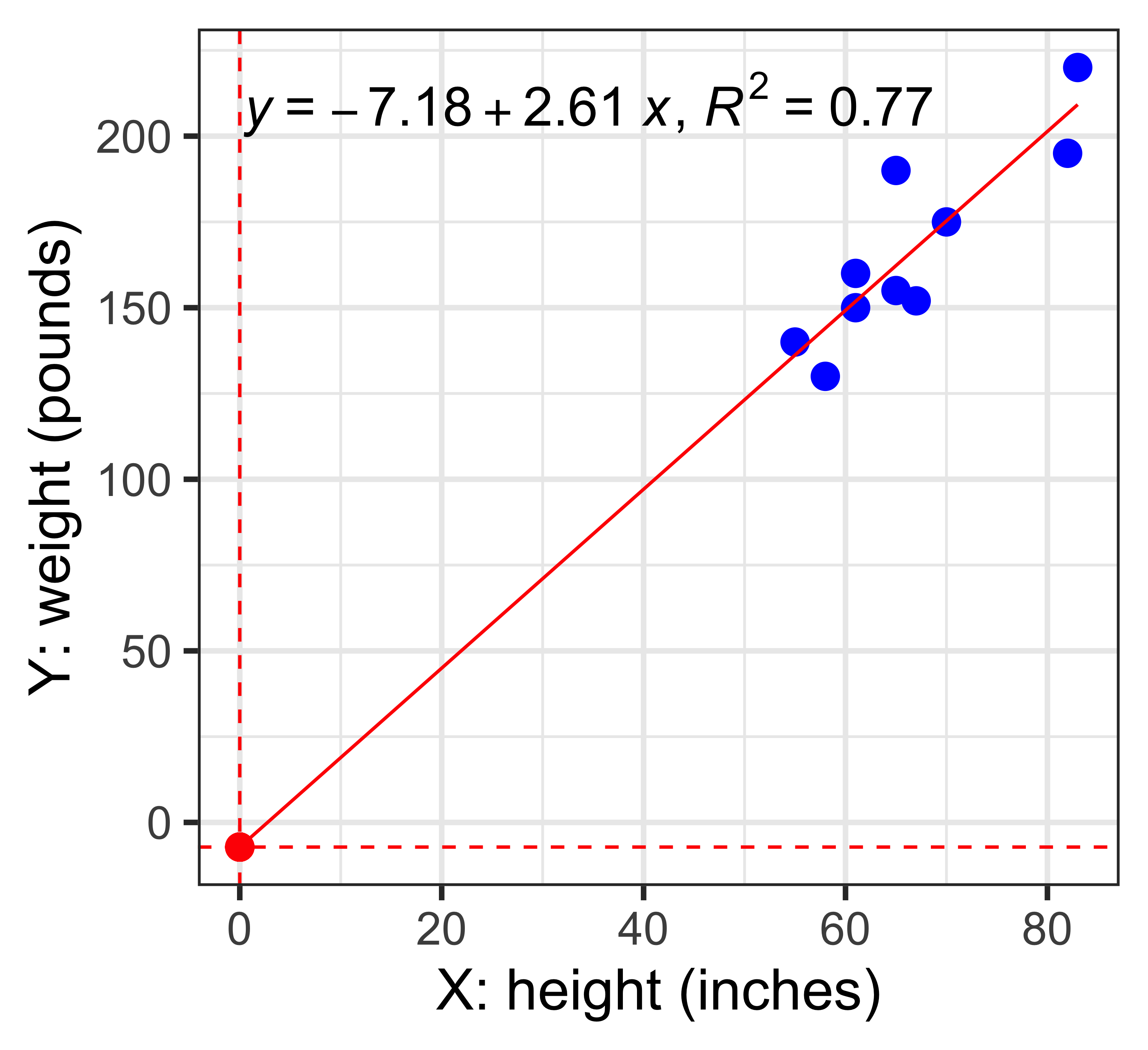
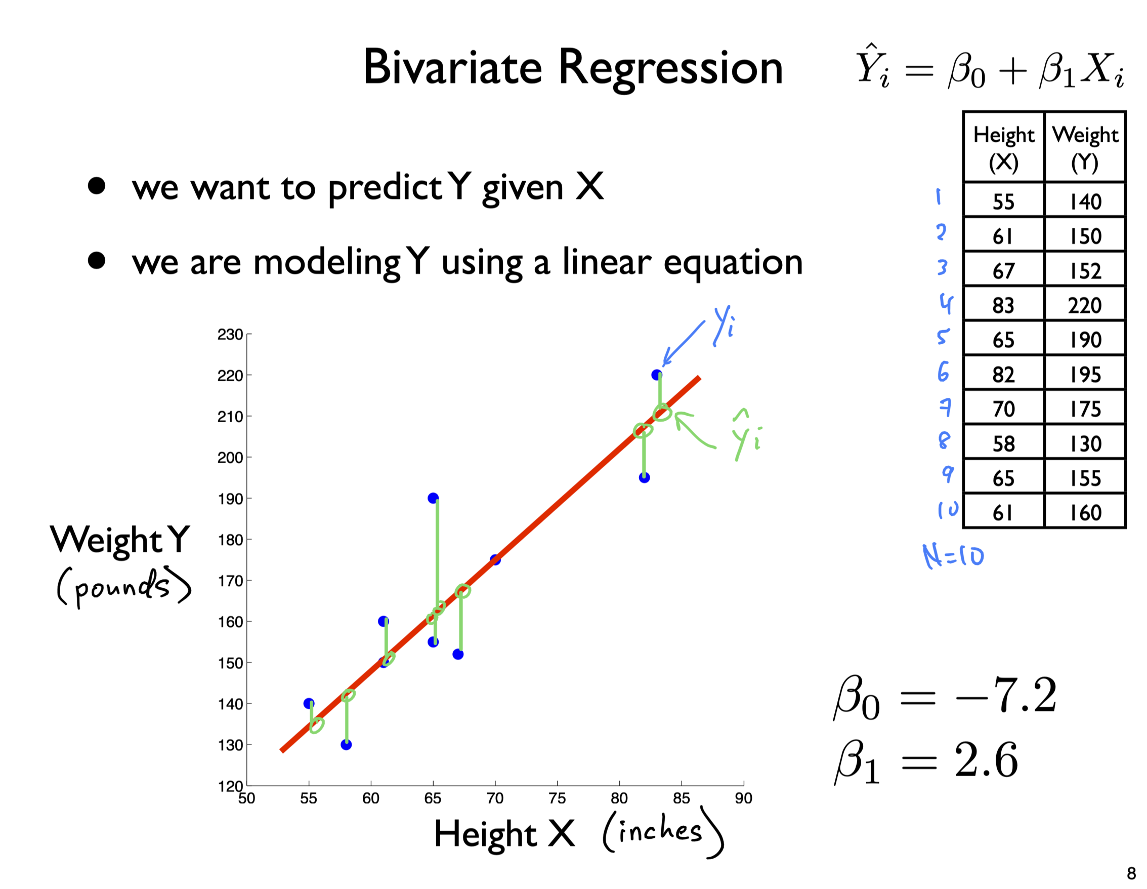
x <- c(55,61,67,83,65,82,70,58,65,61)
y <- c(140,150,152,220,190,195,175,130,155,160)
df <- tibble(x,y)
df

# A tibble: 10 × 2
       x     y
   <dbl> <dbl>
 1    55   140
 2    61   150
 3    67   152
 4    83   220
 5    65   190
 6    82   195
 7    70   175
 8    58   130
 9    65   155
10    61   160

mymod <- lm(y~x, data=df)
coef(mymod)

(Intercept)           x 
  -7.176930    2.606851

Reminders: y-intercept

What does the y-intercept mean?

It is the value where the line crosses the y-axis when x = 0

Reminders: slope

What does the slope mean?

The slope tells you the rate of change.

For every 1 unit of X, Y changes by “slope” amount

E.g., slope = 2.6
then for every 1 unit of X
Y increases by 2.6 units

Regression Equation

Y_{i} = \hat{Y_{i}} + \varepsilon_{i}

\hat{Y}_{i} = \beta_{0} + \beta_{1} X_{i}

\hat{Y}_{i} = estimate of the dependent variable Y_{i}
\beta_{0} = y-intercept of the regression line
\beta_{1} = slope of the regression line
X_{i} = i^{\mathrm{th}} value of the independent variable X
\varepsilon_{i} = i^{\mathrm{th}} residual of the regression line

Quantifying regression fit: R^{2}

Sum of squared residuals is SS_{res} :
Total variability in Y is SS_{tot} :

SS_{res} = \sum_{i}(Y_{i} - \hat{Y}_{i})^{2}
SS_{tot} = \sum_{i}(Y_{i} - \bar{Y})^{2}

Y_{i} are actual values of Y
\hat{Y}_{i} are predicted values of Y using the regression line
\bar{Y} is the mean Y across all observations Y_{i} for i=1 \dots N

Quantifying regression fit: R^{2}

Sum of squared residuals is SS_{res} :
Total variability in Y is SS_{tot} :

SS_{res} = \sum_{i}(Y_{i} - \hat{Y}_{i})^{2}
SS_{tot} = \sum_{i}(Y_{i} - \bar{Y})^{2}

Coefficient of determination R^{2} :

R^{2} = 1 - \frac{SS_{res}}{SS_{tot}}

R^{2} is the proportion of variance in the outcome variable Y that can be accounted for by the predictor variable X

R^{2} always falls between 0.0 and 1.0

Quantifying regression fit: R^{2}

sum of squared residuals = 1.9

sum of squared total = 82.6

R-squared = 0.98

sum of squared residuals = 46.5

sum of squared total = 120.6

R-squared = 0.61

Quantifying regression fit: R^{2}

R^{2} = 0.78
→ 78% of the variance in Y can be accounted for by X
R = 0.22
→ only 4.8% (0.22 x 0.22) of the variance in Y can be accounted for by X

Quantifying regression fit: \sigma_{est}

\sigma_{est} is the standard error of the estimate
\sigma_{est} is a measure of accuracy of predicting Y using X
whereas R^{2} is always between 0.0 and 1.0,
→ \sigma_{est} is in units of Y, the predicted variable
this makes \sigma_{est} a useful measure of model fit

Quantifying regression fit: \sigma_{est}

\sigma_{est} = \sqrt{\frac{\sum(Y-\hat{Y})^{2}}{N}}

\sigma_{est} is a measure of accuracy of predicting Y using X
\sigma_{est} is in units of Y, the predicted variable

Quantifying regression fit: \sigma_{est}

\sigma_{est} = \sqrt{\frac{\sum(Y-\hat{Y})^{2}}{N}}

\sigma_{est} is for a population
For a sample the notation is s_{est}

Quantifying regression fit: s_{est}

For a sample the notation is s_{est}

s_{est} = \sqrt{\frac{\sum_{i}(Y_{i}-\hat{Y}_{i})^{2}}{N-2}}

N-2 because we estimate 2 parameters from our sample (slope and intercept of regression line)

Quantifying regression fit: s_{est}

Y = -7.2 + 2.6 X
R^{2} = 0.772
s_{est} = 14.11 (pounds)

Prediction

predict values of y given:
- a new value of x
- the regression equation

Prediction

for a person with height = 75 inches
→ what is their weight?
regression equation:
weight = -7.18 + (2.61 * height)
weight = -7.18 + (2.61 * 75)
weight = -7.18 + 195.75
weight = 188.57 pounds
from summary() of our lm() in R:
s_{est} = 14.11 pounds

Prediction

for a person with height = 57 inches
→ what is their weight?
regression equation:
weight = -7.18 + (2.61 * height)
weight = -7.18 + (2.61 * 57)
weight = -7.18 + 148.77
weight = 141.59 pounds
from summary() of our lm() in R:
s_{est} = 14.11 pounds

Prediction

for a person with height = 0 inches
→ what is their weight?
regression equation:
weight = -7.18 + (2.61 * height)
weight = -7.18 + (2.61 * 0) weight = -7.18 + 0
weight = -7.18 pounds
???
predictions are only valid within the range of observed data
extrapolate at your own risk!

Confidence Intervals

another way of characterizing the precision of estimates
- of model coefficients (slope, intercept)
- of model prediction (predicted Y given new X)
95% CI

Confidence Intervals

let’s first quickly review confidence intervals of the mean of a sample before we talk about confidence intervals of regression coefficients

Confidence Intervals

recall* that the 95% CI of the mean of a sample is:

\bar{X} \pm t_{(0.975,N-1)} \left( \frac{s}{\sqrt{N}} \right)

x <- c(55,61,67,83,65,82,70,58,65,61)
N <- length(x)
ci_lower <- mean(x) - (qt(.975,N-1) * (sd(x)/sqrt(N)))
ci_upper <- mean(x) + (qt(.975,N-1) * (sd(x)/sqrt(N)))
(mean(x))

[1] 66.7

(c(ci_lower, ci_upper))

[1] 59.98047 73.41953

Confidence Intervals

recall* that the 95% CI of the mean of a sample is:

\bar{X} \pm t_{(0.975,N-1)} \left( \frac{s}{\sqrt{N}} \right)

x <- c(55,61,67,83,65,82,70,58,65,61)
library(lsr) # you may need to install this package
ciMean(x, 0.95)

      2.5%    97.5%
x 59.98047 73.41953

Confidence Intervals

95% CI of the mean of our sample is (59.98, 73.42)
how to interpret* this?
95% chance the population mean is between 59.95 and 73.42
→ nope … but (subtly) close! → the “95% chance” is a statement about the confidence interval, not about the population mean

Confidence Intervals

95% CI of the mean of our sample is (59.98, 73.42)
If we replicated the experiment over and over again, and computed a 95% confidence interval for each replication, then 95% of those confidence intervals would contain the population mean
(but we will never know which ones!)

Confidence Intervals

recall our regression model:
Y = -7.18 + 2.61 X
- \beta_{0}=-7.18
- \beta_{1}=2.61
we can also compute 95% CIs for coefficients (\beta_{0},\beta_{1})

Confidence Intervals

CI(b) = \hat{b} \pm \left( t_{crit} \times SE(\hat{b}) \right)

\hat{b} is each coefficient in the regression model
t_{crit} is the critical value of t
SE(\hat{b}) is the standard error of the regression coefficient

in R it’s easy, use confint():

d <- tibble(x=c(55,61,67,83,65,82,70,58,65,61),
            y=c(140,150,152,220,190,195,175,130,155,160))
mymod <- lm(y ~ x, data = d)
coef(mymod)

(Intercept)           x 
  -7.176930    2.606851

confint(mymod)

                 2.5 %    97.5 %
(Intercept) -84.898712 70.544852
x             1.451869  3.761832

Confidence Intervals

d <- tibble(x=c(55,61,67,83,65,82,70,58,65,61),
            y=c(140,150,152,220,190,195,175,130,155,160))
mymod <- lm(y ~ x, data = d)
coef(mymod)

(Intercept)           x 
  -7.176930    2.606851

confint(mymod)

                 2.5 %    97.5 %
(Intercept) -84.898712 70.544852
x             1.451869  3.761832

interpretation of regression coefficient CIs is the same:
If we were to replicate our sample a bunch of times, by resampling from the population and fitting a new regression model each time, and compute confidence intervals for the regression coefficients each time, then 95% of those CIs would contain the population value of the coefficients.

Hypothesis tests for Regression

F(1,8)=27.09
p=0.0008176
→ what is this hypothesis test of?

Hypothesis tests for Regression

This is a test of the model “as a whole”*
specifically a test of the “full” regression model versus a “restricted” version of the model in which there is no dependence of Y on X
- (i.e. the slope \beta_{1} is zero)
in this way the hypothesis test is essentially a test of whether \beta_{1}=0 or not
Y = \beta_{0} + \beta_{1} X : full model (our alternate hypothesis H_{1})
Y = \beta_{0} : restricted model (our null hypothesis H_{0})

Hypothesis tests for Regression

F test of model as a whole tests full model vs restricted model
Y = \beta_{0} + \beta_{1} X : full
Y = \beta_{0} : restricted
When there is only one dependent variable (X) in the regression model, (and hence only one slope \beta_{1}), then this is equivalent to a test of whether the slope is zero

Hypothesis tests for Regression

also: hypothesis tests on model coefficients
null hypothesis H_{0}: coefficient = zero
alternate hypothesis H_{1}: coefficient is not zero
intercept (\beta_{0}): p = 0.836700
slope (\beta_{1}): p = 0.000818

Hypothesis tests for Regression

intercept (\beta_{0}) = -7.1769
p = 0.836700
slope (\beta_{1}) = 2.6069
p = 0.000818
what do these p-values mean precisely?

Hypothesis tests for Regression

intercept (\beta_{0}) = -7.1769
p = 0.836700
Under the null hypothesis H_{0} the probability of obtaining an intercept as large (farthest from zero) as -7.1769 due to random sampling is 83.67%
That is pretty high! We cannot really reject H_{0}
We cannot reject H_{0} (that the intercept = zero)
We infer that the intercept is most likely = zero

Hypothesis tests for Regression

slope (\beta_{1}) = 2.6069
p = 0.000818
Under the null hypothesis H_{0} the probability of obtaining a slope as large (farthest from zero) as 2.6069 due to random sampling is 0.0818%
That is pretty low! We will reject H_{0} that the slope is zero
The slope is not zero. What is it?
Our estimate of the slope is \beta_{1} = 2.6069
Our 95% confidence interval is [1.451869, 3.761832] from confint()

Assumptions of Linear Regression

Linearity: linear relationship between X and Y
Normality: (nearly) normally distributed residuals
Homoscedasticity: Constant variance of Y across the range of X
Outliers: no extreme outliers
Independence: observations are independent of each other

1. Linearity

relationship between the predictor variable (X) and the predicted variable (Y) should be linear
check with a scatterplot either of the data or residuals

2. Normality

the residuals should be nearly normally distributed
can check using a histogram of the residuals:

2. Normality

the residuals should be nearly normally distributed
can also check using a Q-Q plot:

2. Normality

statistical test for normality: shapiro.test() (Shapiro-Wilk test)
null hypothesis H_{0}: data are normally distributed
alternate hypothesis H_{1}: data are not normally distributed
p < .05: reject the null hypothesis
- conclude data are not normally distributed
test the residuals: shapiro.test(residuals(my.mod))

3. Homoscedasticity

homogeneity of variance
variance of Y is the same across the range of X values
plot X vs Y data:

3. Homoscedasticity

homogeneity of variance
variance of Y is the same across the range of X values
or: plot X vs Residuals (Y-\hat{Y})

3. Homoscedasticity

statistical test for homoscedasticity: bptest() (Breusch-Pagan test)
in the car package: ncvTest() (non-constant variance test)
null hypothesis H_{0}: homoscedasticity
alternate hypothesis H_{1}: heteroscedasticity
p < .05: reject the null hypothesis
- conclude data are heteroscedastic
apply the ncvTest() to the lm() model object: ncvTest(my.mod)

4. Outliers

we should not fit our linear model to a dataset that includes extreme outliers

4. Outliers

Cook’s distance is one quantitative way of identifying observations that have a disproportionate influence on the regression line
see Navarro text section 15.9

Violations: what to do?

Linearity: If your data are not linear don’t model it using a linear model! Non-linear methods do exist.
Normality: if severe, consider transforming the dependent variable, e.g. using logarithm, square root, Box-Cox transformation, etc.
Homoscedasticity: could consider transforming the dependent variable; could also use weighted regression
Outliers: remove them!

Multiple Regression

Multiple Regression

In bivariate regresssion we use X to predict Y:
- Y_{i} = \beta_{0} + \beta_{1} X + \varepsilon_{i}
- one dependent variable Y (the variable to be predicted)
- one independent variable X (the variable we are using to predict Y)
- N different observations of each (X_{i},Y_{i}), for i=1 \dots N
- two model coefficients, \beta_{0} (intercept) & \beta_{1} (slope)

Multiple Regression

In Multiple Regression: we use N predictor variables X_{1}, X_{2}, \dots X_{N} to predict Y
- Y_{i} = \beta_{0} + \beta_{1} X_{i1} + \beta_{2} X_{i2} + \dots + \beta_{k} X_{ik} +\varepsilon_{i}
- one dependent variable Y (the variable to be predicted)
- K independent variables X_{k}, for k=1 \dots K
- N different observations (X_{i},Y_{i}), for i=1 \dots N
- k+1 model coefficients \beta (one slope for each X_{i} plus a model intercept \beta_{0})
Y_{i} = \beta_{0} + \displaystyle\sum_{k=1}^{K} \left( \beta_{k} X_{ik} \right) +\varepsilon_{i}

1 predictor

Y_{i} = \beta_{0} + \beta_{1} X + \varepsilon_{i}
one dependent variable Y (the variable to be predicted)
one independent variable X (the variable we are using to predict Y)
N different observations of each (X_{i},Y_{i}), for i=1 \dots N
two model coefficients, \beta_{0} (intercept) & \beta_{1} (slope)

2 predictors

Y_{i} = \beta_{0} + \beta_{1} X_{i1} + \beta_{2} X_{i2} +\varepsilon_{i}
Model a car’s fuel efficiency (MPG) as a function of:
- the weight of the car
- the car’s engine size
Y: MPG of cars
X_{1}: car weight
X_{2}: engine size
\beta_{1}: dependence of (slope of) MPG (Y) on car weight (X_{1})
\beta_{2}: dependence of (slope of) MPG (Y) on engine size (X_{2})
\beta_{0}: intercept — predicted MPG (Y) when car weight and engine size are both zero

2 predictors

Y_{i} = \beta_{0} + \beta_{1} X_{i1} + \beta_{2} X_{i2} +\varepsilon_{i}
MPG ~ Weight + Displacement (using the mtcars built-in dataset)

2 predictors

Y_{i} = \beta_{0} + \beta_{1} X_{i1} + \beta_{2} X_{i2} +\varepsilon_{i}
MPG ~ Weight + Displacement

2 predictors

Y_{i} = \beta_{0} + \beta_{1} X_{i1} + \beta_{2} X_{i2} +\varepsilon_{i}
MPG ~ Weight + Displacement
value of \beta_{1}: MPG dependency (slope) on Weight

2 predictors

Y_{i} = \beta_{0} + \beta_{1} X_{i1} + \beta_{2} X_{i2} +\varepsilon_{i}
MPG ~ Weight + Displacement
value of \beta_{2}: MPG dependency (slope) on Displacement

K predictors

Y_{i} = \beta_{0} + \displaystyle\sum_{k=1}^{K} \left( \beta_{k} X_{ik} \right) +\varepsilon_{i} - sorry! I can’t draw in > 3 dimensions

Next Week: More on multiple regression

Linear Regression II & Intro to Multiple Regression

scatterplot plus regression line

R: intercept and slope

Reminders: y-intercept

Reminders: slope

Regression Equation

Quantifying regression fit: R^{2}

Quantifying regression fit: R^{2}

Quantifying regression fit: R^{2}

Quantifying regression fit: R^{2}

Quantifying regression fit: \sigma_{est}

Quantifying regression fit: \sigma_{est}

Quantifying regression fit: \sigma_{est}

Quantifying regression fit: s_{est}

Quantifying regression fit: s_{est}

Prediction

Prediction

Prediction

Prediction

Confidence Intervals

Confidence Intervals

Confidence Intervals

Confidence Intervals

Confidence Intervals

Confidence Intervals

Confidence Intervals

Confidence Intervals

Confidence Intervals

Hypothesis tests for Regression

Hypothesis tests for Regression

Hypothesis tests for Regression

Hypothesis tests for Regression

Hypothesis tests for Regression

Hypothesis tests for Regression

Hypothesis tests for Regression

Assumptions of Linear Regression

1. Linearity

2. Normality

2. Normality

2. Normality

3. Homoscedasticity

3. Homoscedasticity

3. Homoscedasticity

4. Outliers

4. Outliers

Violations: what to do?

Next

Multiple Regression

Multiple Regression

1 predictor

2 predictors

2 predictors

2 predictors

2 predictors

2 predictors

K predictors

Next