Correlations between two variables can occur by chance, and be completlely meaningless
we will do some simulations!
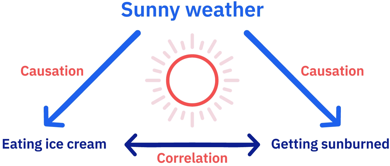
5 Third variable
5 Third variable
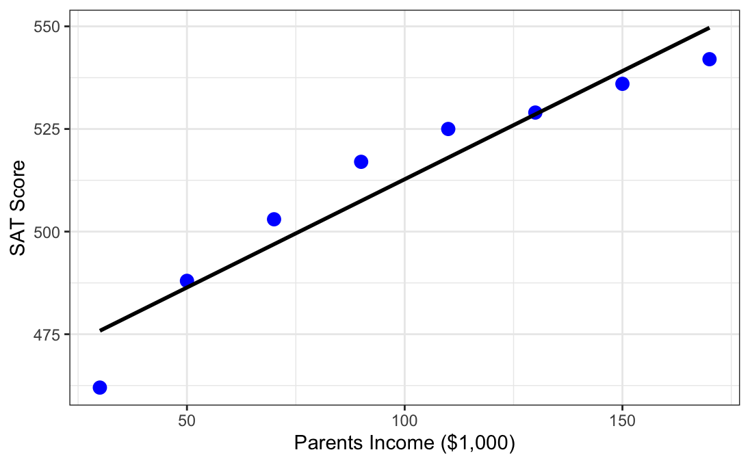
Molly’s parents’ income is $50k
Molly takes the SAT on Monday and scores a 480
on Thursday Mom gets a new job, the new income is $150k
If Molly re-takes the SAT on Friday, will her Mom’s increased income cause her to score 53 points higher? (0.53 * $100k)
SAT = 460 + 0.53 ($inc)
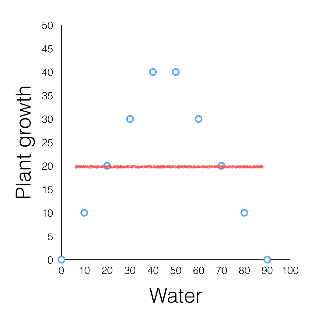
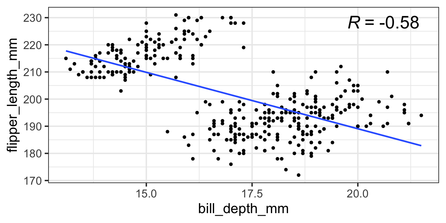
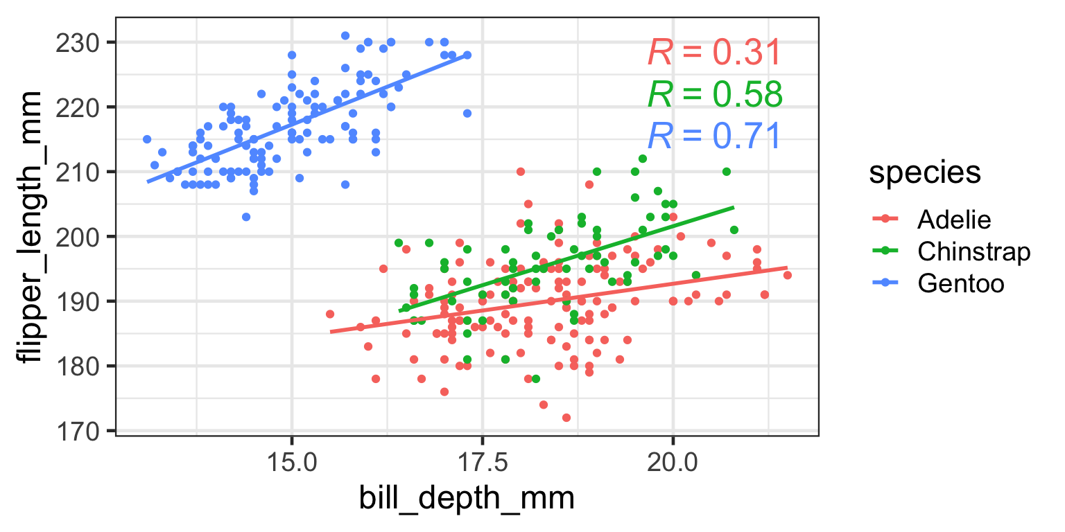
Simpson’s Paradox
a trend appears in several groups of data but disappears or reverses when the groups are combined
Simpson’s Paradox
a trend appears in several groups of data but disappears or reverses when the groups are combined
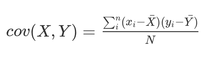
Correlation and variance
r can be between [-1,1]
r^2 is always between [0,1]
r^{2} is the proportion of variance in one variable that is explained by the other variable
r=0.5 means that 25% of the variance in one variable is explained by the other variable
r=0.1 means that only 1% of the variance in one variable is explained by the other variable
(99% of the variance is unexplained by the other variable)
Correlations and Random Chance
What is randomness?
Two related ideas:
Things have equal chance of happening (e.g., a coin flip)
50% heads, 50% tails
Correlations and Random Chance
What is randomness?
Two related ideas:
Independence: One thing happening is totally unrelated to whether another thing happens
the outcome of one flip doesn’t predict the outcome of another
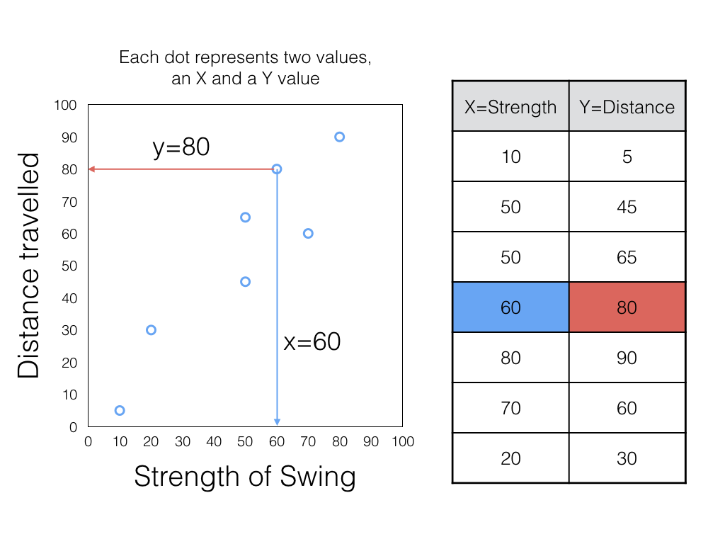
Two random variables
On average there should be zero correlation between two variables containing randomly drawn numbers
The numbers in variable X are drawn randomly (independently), so they do not predict numbers in Y
The numbers in variable Y are drawn randomly (independently), so they do not predict numbers in X
Two random variables
If X can’t predict Y, then correlation should be 0 right?
on average yes
for individual samples, no!
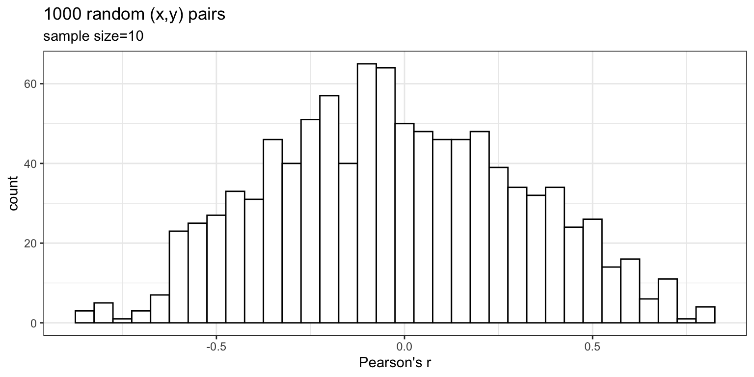
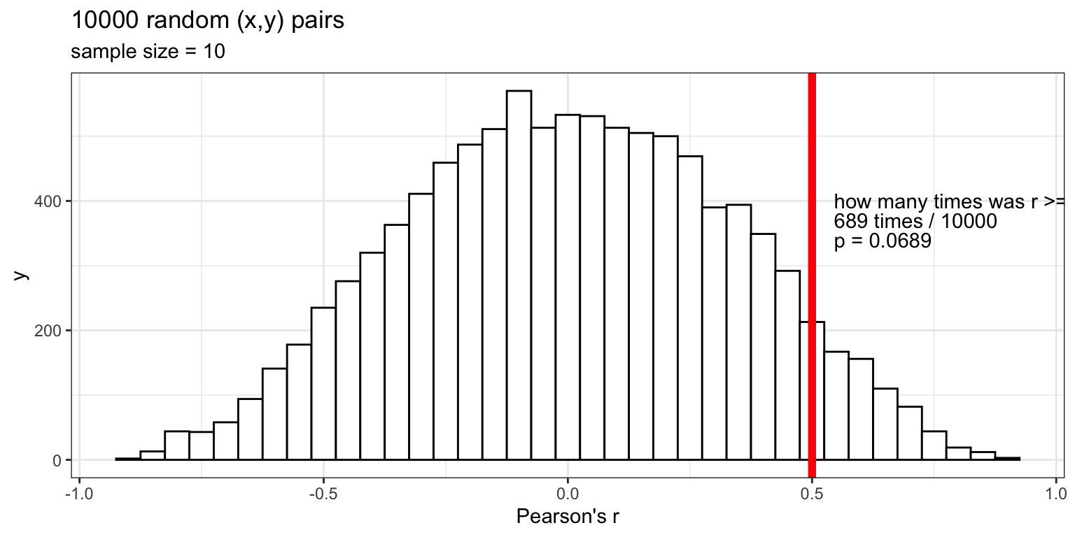
R: random numbers
In R, runif() allows you to sample random numbers (uniform distribution) between a min and max value. Numbers in the range have an equal chance of occuring
We can see that randomly sampling numbers can produce a range of correlations, even when there shouldn’t be a “correlation”
What is the average correlation produced by chance? (zero)
What is the range of correlations that chance can produce?
Simulating what chance can do
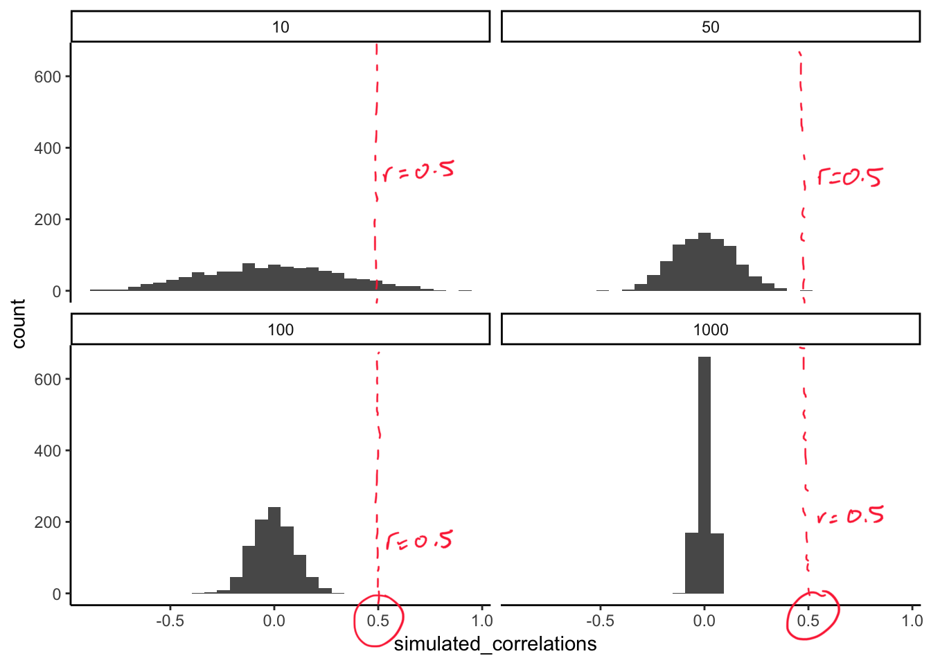
The role of sample size (N)
The range of chance correlations decreases as N increases
The inference problem
Let’s say we sampled some data, and we found a correlation, (r = 0.5)
BUT: We know chance can sometimes produce random correlations
The inference problem
Is the correlation we observed in the sample a reflection of a real correlation in the population?
Is one variable really related to the other?
Or, is there really no correlation between these two population variables?
i.e. the correlation in the sample is spurious
i.e. it was produced by chance through random sampling → this is H_{0}, the null hypothesis
The (simulated) Null Hypothesis
Making inferences about chance
In a sample of size N=10, we observe: r=0.5
Null Hypothesis H_{0}:
→ no correlation actually exists in the population
→ actual population correlation r=0.0
Alternative Hypothesis H_{1}: correlation does exist in the population, and r=0.5 is our best estimate
We don’t know what the truth actually is
Making inferences about chance
We can only make an inference based on:
What is the probability p of observing:
→ an r in a sample as big as r=0.5
→ in a sample of size N=10
→ under the null hypothesis H_{0} in which the populationr=0.0
Making inferences about chance
If that probability p is low enough:
→ we conclude that it is an unlikely scenario
→ and we reject H_{0}
Making inferences about chance
How low can you go?
If that probability p is low enough:
→ we conclude that it is an unlikely scenario
→ and we reject H_{0}
How low is low enough?
p < .05
p < .01
p < .001
Making inferences about chance
cor.test() in R will give you the probability p of obtaining a sample correlation as large as you did under the null hypothesis where the population correlation is actually zero
Assumptions:
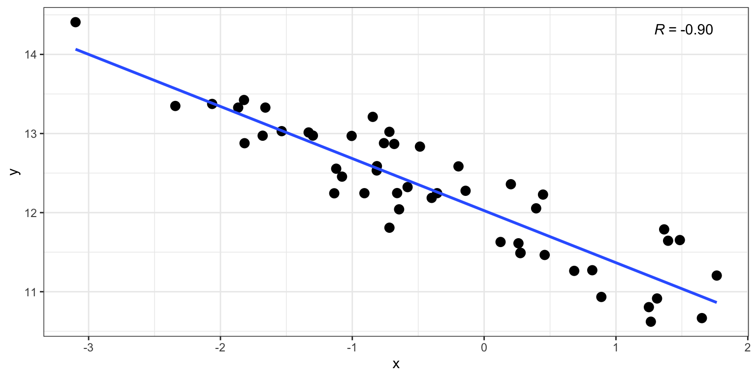
→ x vs y is a linear relationship (plot it!)
→ x & y variables are normally distributed (shapiro.test())
    Shapiro-Wilk normality test

data:  x
W = 0.97589, p-value = 0.3943
shapiro.test(y)
    Shapiro-Wilk normality test

data:  y
W = 0.97548, p-value = 0.3808
Making inferences about chance
cor.test(x, y)
    Pearson's product-moment correlation

data:  x and y
t = -14.55, df = 48, p-value < 2.2e-16
alternative hypothesis: true correlation is not equal to 0
95 percent confidence interval:
 -0.9439854 -0.8341607
sample estimates:
       cor
-0.9028732
Making inferences about chance
if normality assumption is not met, you can use Spearman’s rank correlation coefficient \rho (“rho”)
See Chapter 5.7.6 of Navarro “Learning Statistics with R”
cor.test(x, y, method="spearman")
    Spearman's rank correlation rho

data:  x and y
S = 39340, p-value < 2.2e-16
alternative hypothesis: true rho is not equal to 0
sample estimates:
       rho
-0.8890756
IMPORTANT: “significant” \neq “large”
significance test is not whether r is large
test is whether r is “statistically significant”
whether r is reliably different than 0.0
IMPORTANT: “significant” \neq “large”
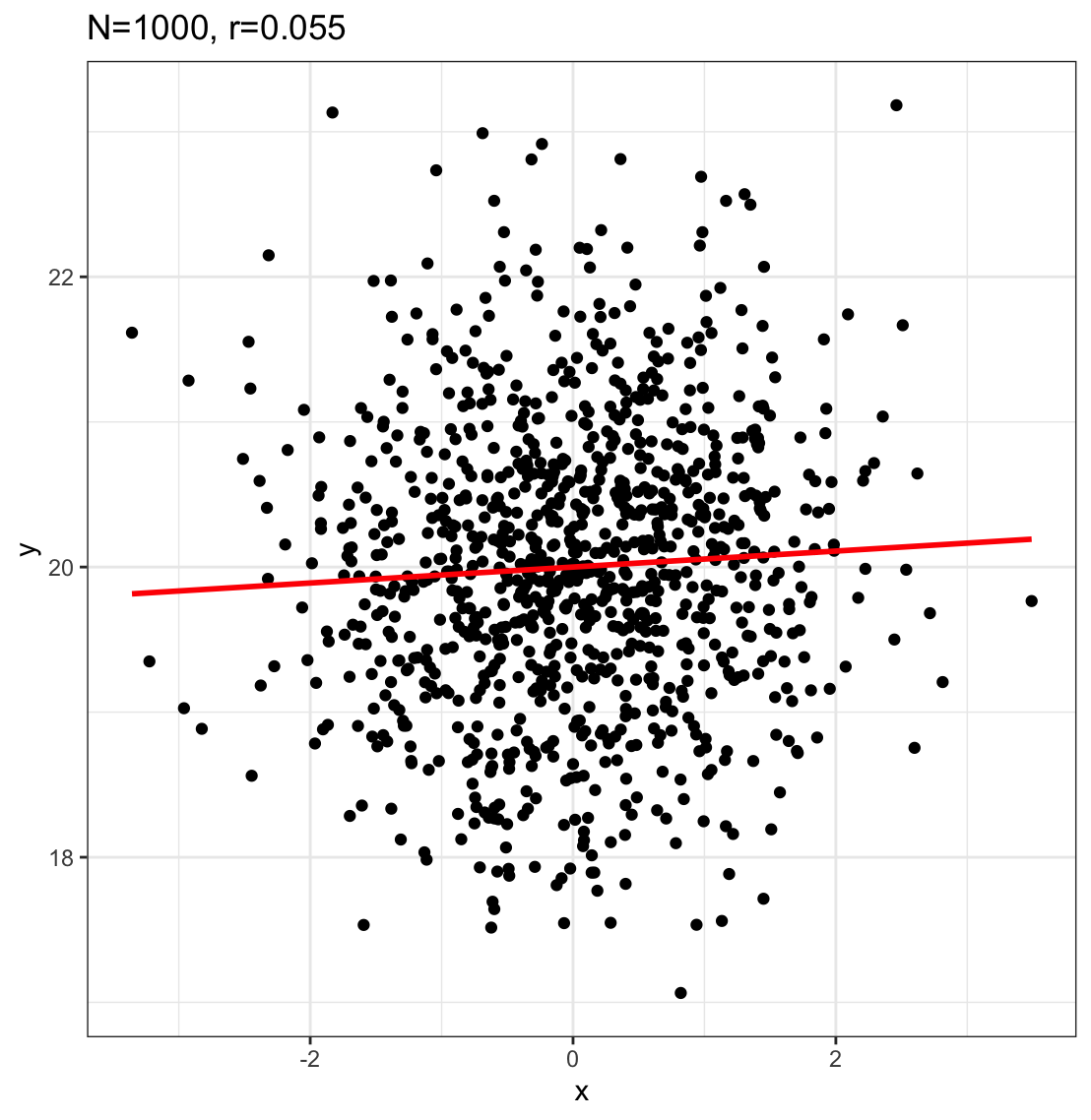
N=1000
r=0.055
p = 0.041
is r significant? (yes)
is r large? (no)
r^{2}= .055*.055 = .003025
= 0.3\% variance explained
99.7\% of the variance is unexplained
IMPORTANT: “significant” \neq “large”
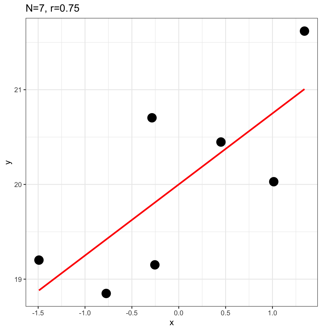
N=7
r=0.75
p = 0.052
is r significant? (no)
is r large? (yes)
NEXT
Linear Regression
Linear Regression
geometric interpretation of correlation
can be used for prediction
a linear model relating one variable to another variable
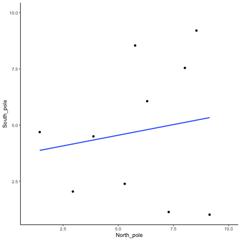
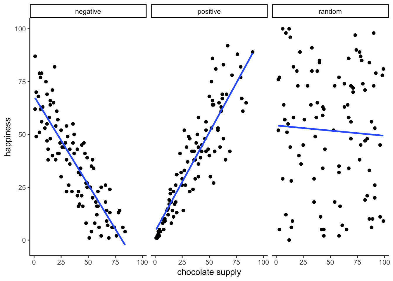
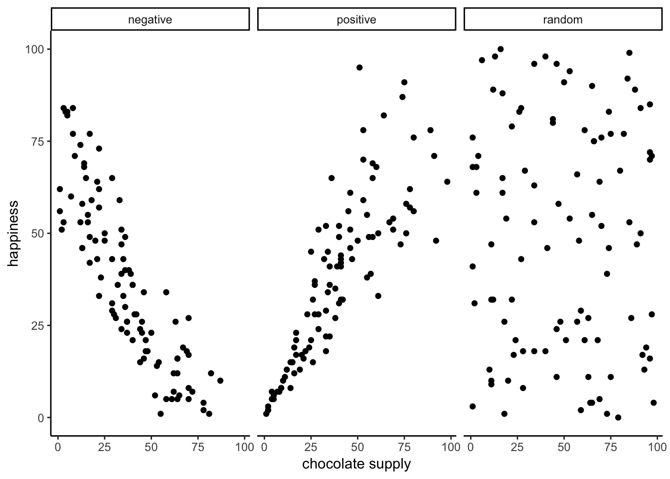
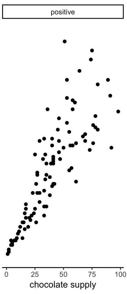
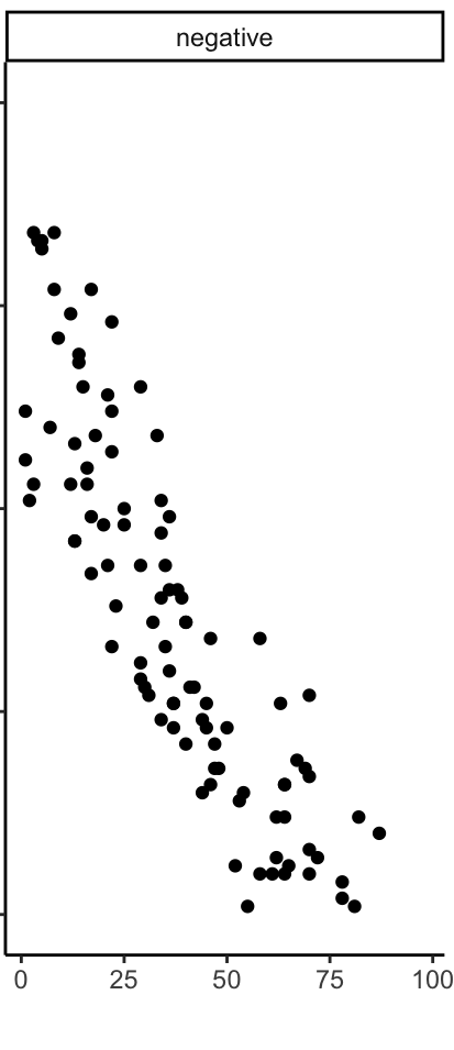
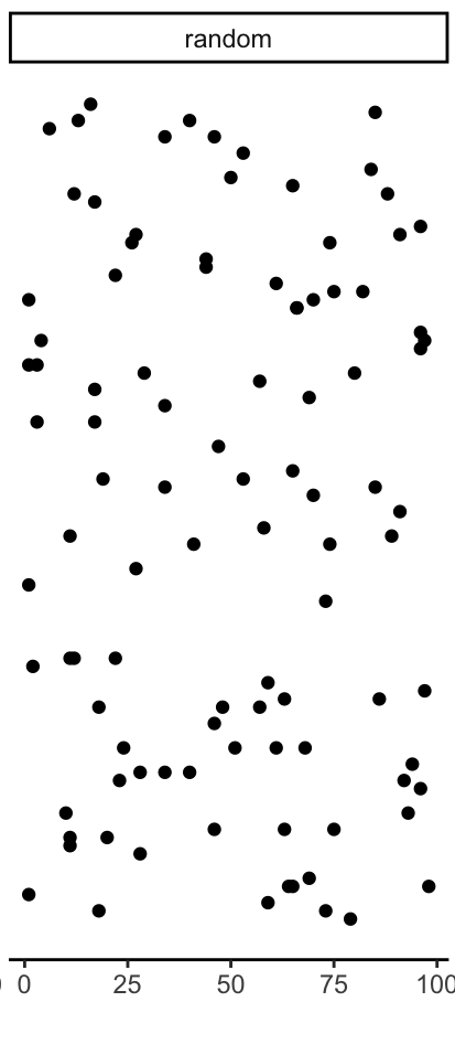
Examples of correlation
Correlation with Regression lines
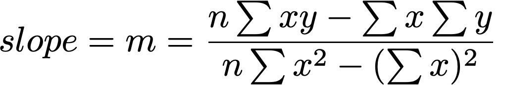
What is a regression line?
first: it’s a line (we will need the equation)
the best fit line
how do we determine which line fits best?
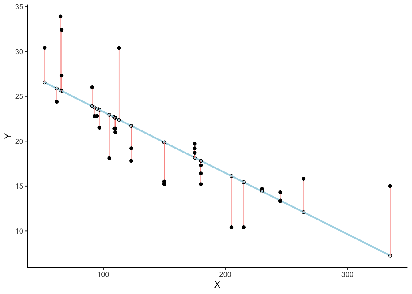
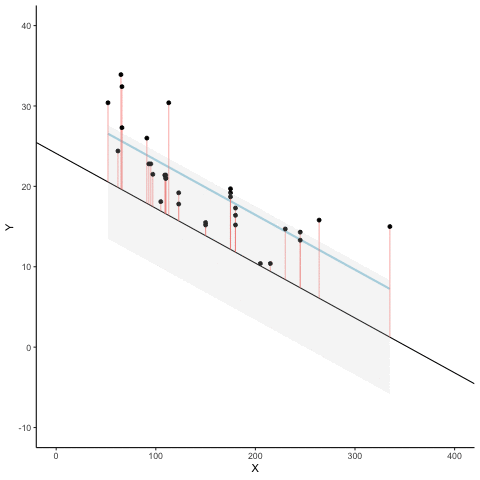
Residuals and error
What is a regression line?
first: it’s a line (we will need the equation)
the best fit line
how do we determine which line fits best?
The regression line minimizes the sum of the (squared) residuals
Animated Residuals
regression minimizes the sum of the (squared) residuals
Finding the best fit line
how do we find the best fit line?
First step, remember what lines are …
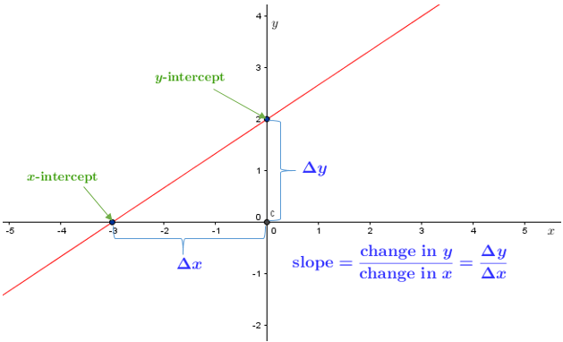
Equation for a line
y = mx +b
y = \text{slope}*x + \text{yintercept}
y = value on y-axis
m = slope of the line
x = value on x-axis
b = value on y-axis when x = 0
We will also use this form:
y = \beta_{0} + \beta_{1}x
solving for y
predicting y based on x
y = .5x + 2
What is the value of y, when x is 0?
y = .5*0 + 2 y = 0+2 y = 2
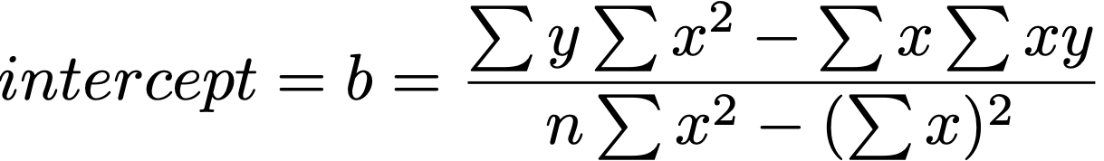
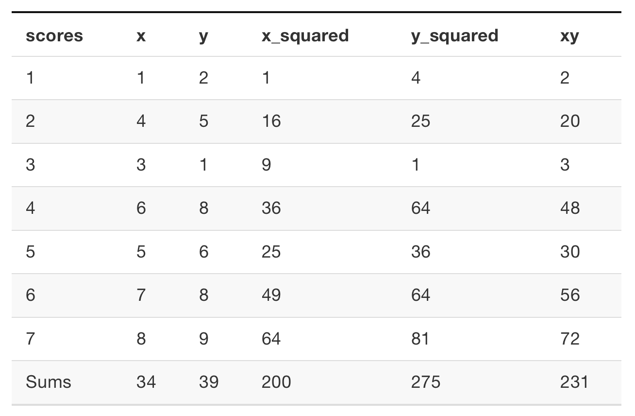
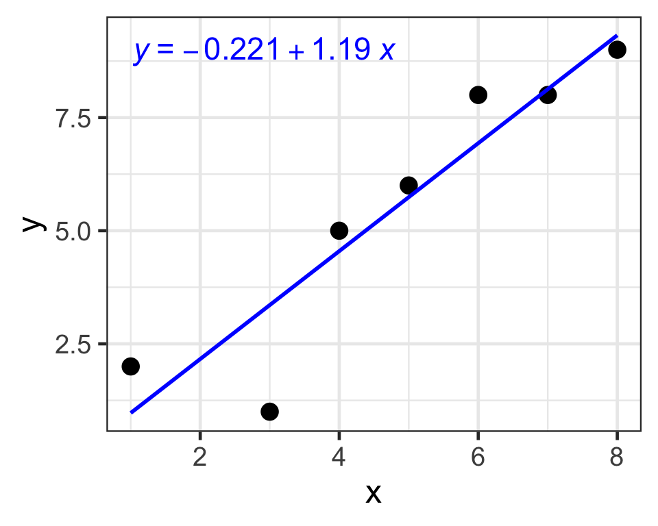
Finding the best fit line
find m and b for:
Y = mX + b
so that the regression line minimizes the sum of the squared residuals

 SAT = 460 + 0.53 ($inc)

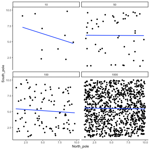
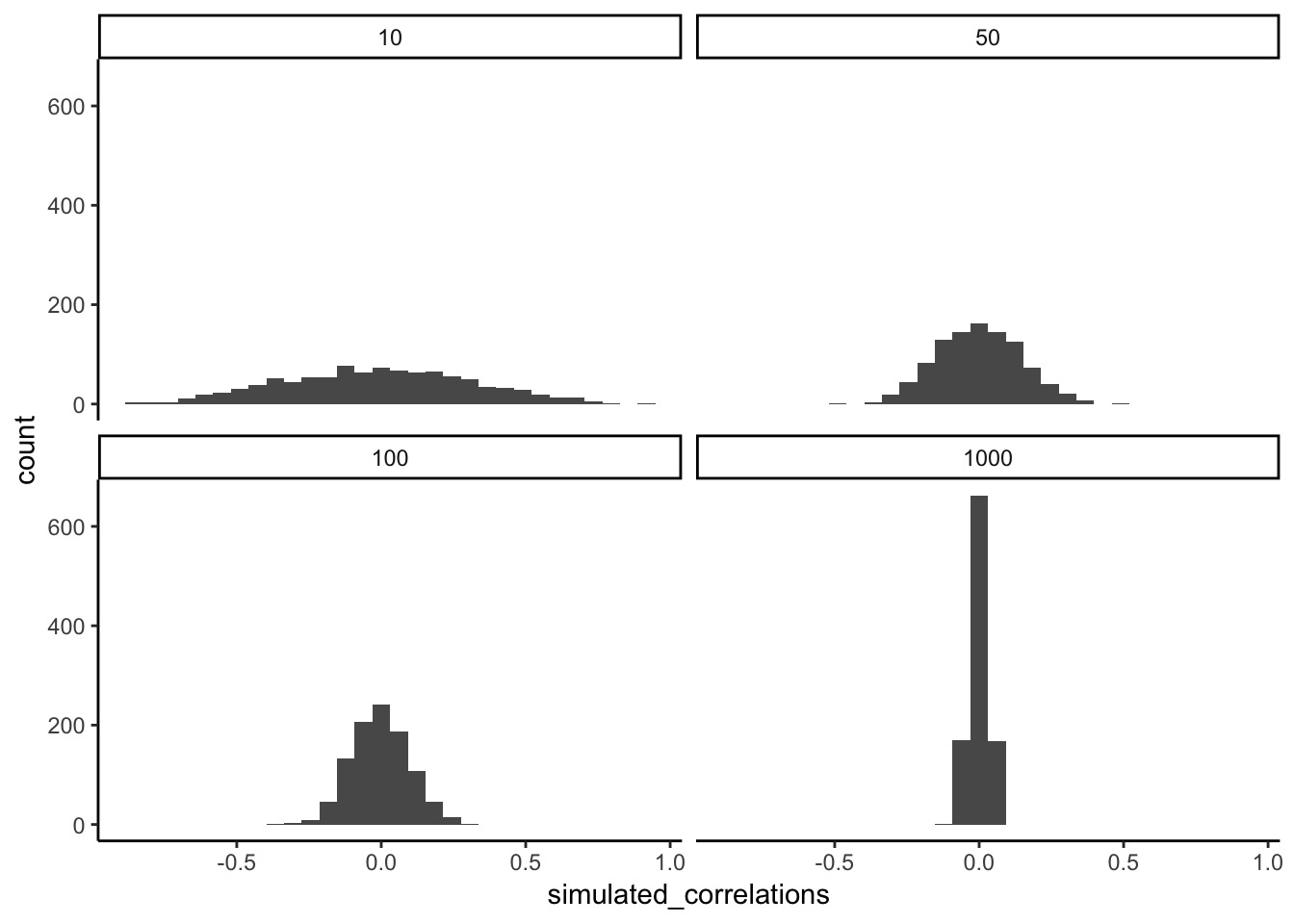 The range of chance correlations decreases as N increases