Data wrangling & visualization II — dplyr

Week 3

Midterm & Final Exam Format

closed-book
no laptop, no calculators
1 cheat-sheet permitted (1 double-sided letter-sized sheet)
multiple choice
short-answer Qs
data visualization & interpretation
statistical tests & interpretation
generally very similar to the homeworks

Data Transformation

rarely do we get data in exactly the format we need
create new variables
create summaries of variables (counts, means, sds)
rename variables
reorder variables
lots more!

The `dplyr` package

core package of the tidyverse
https://dplyr.tidyverse.org/
a grammar of data manipulation

The `dplyr` package

provides a set of verbs that help you manipulate data

The `nycflights13` dataset

https://github.com/tidyverse/nycflights13
- all flights that departed from New York City area airports in 2013
- to destinations in the USA, Puerto Rico, and the American Virgin Islands
33,776 flights in total
contains 5 separate data tables
- flights: all flights departing NYC in 2013—today we will use this
- weather: hourly meterological data for each airport
- planes: construction info about each plane
- airports: airport names and locations
- airlines: translation between two-letter airline codes and names

Install the `nycflights13` package

only have to do this once

install.packages("nycflights13")

Load required packages

must do this each time you start RStudio

library(nycflights13)
library(tidyverse)

`flights`

flights

# A tibble: 336,776 × 19
    year month   day dep_time sched_dep_time dep_delay arr_time sched_arr_time
   <int> <int> <int>    <int>          <int>     <dbl>    <int>          <int>
 1  2013     1     1      517            515         2      830            819
 2  2013     1     1      533            529         4      850            830
 3  2013     1     1      542            540         2      923            850
 4  2013     1     1      544            545        -1     1004           1022
 5  2013     1     1      554            600        -6      812            837
 6  2013     1     1      554            558        -4      740            728
 7  2013     1     1      555            600        -5      913            854
 8  2013     1     1      557            600        -3      709            723
 9  2013     1     1      557            600        -3      838            846
10  2013     1     1      558            600        -2      753            745
# ℹ 336,766 more rows
# ℹ 11 more variables: arr_delay <dbl>, carrier <chr>, flight <int>,
#   tailnum <chr>, origin <chr>, dest <chr>, air_time <dbl>, distance <dbl>,
#   hour <dbl>, minute <dbl>, time_hour <dttm>

`flights`

glimpse(flights)

Rows: 336,776
Columns: 19
$ year           <int> 2013, 2013, 2013, 2013, 2013, 2013, 2013, 2013, 2013, 2…
$ month          <int> 1, 1, 1, 1, 1, 1, 1, 1, 1, 1, 1, 1, 1, 1, 1, 1, 1, 1, 1…
$ day            <int> 1, 1, 1, 1, 1, 1, 1, 1, 1, 1, 1, 1, 1, 1, 1, 1, 1, 1, 1…
$ dep_time       <int> 517, 533, 542, 544, 554, 554, 555, 557, 557, 558, 558, …
$ sched_dep_time <int> 515, 529, 540, 545, 600, 558, 600, 600, 600, 600, 600, …
$ dep_delay      <dbl> 2, 4, 2, -1, -6, -4, -5, -3, -3, -2, -2, -2, -2, -2, -1…
$ arr_time       <int> 830, 850, 923, 1004, 812, 740, 913, 709, 838, 753, 849,…
$ sched_arr_time <int> 819, 830, 850, 1022, 837, 728, 854, 723, 846, 745, 851,…
$ arr_delay      <dbl> 11, 20, 33, -18, -25, 12, 19, -14, -8, 8, -2, -3, 7, -1…
$ carrier        <chr> "UA", "UA", "AA", "B6", "DL", "UA", "B6", "EV", "B6", "…
$ flight         <int> 1545, 1714, 1141, 725, 461, 1696, 507, 5708, 79, 301, 4…
$ tailnum        <chr> "N14228", "N24211", "N619AA", "N804JB", "N668DN", "N394…
$ origin         <chr> "EWR", "LGA", "JFK", "JFK", "LGA", "EWR", "EWR", "LGA",…
$ dest           <chr> "IAH", "IAH", "MIA", "BQN", "ATL", "ORD", "FLL", "IAD",…
$ air_time       <dbl> 227, 227, 160, 183, 116, 150, 158, 53, 140, 138, 149, 1…
$ distance       <dbl> 1400, 1416, 1089, 1576, 762, 719, 1065, 229, 944, 733, …
$ hour           <dbl> 5, 5, 5, 5, 6, 5, 6, 6, 6, 6, 6, 6, 6, 6, 6, 5, 6, 6, 6…
$ minute         <dbl> 15, 29, 40, 45, 0, 58, 0, 0, 0, 0, 0, 0, 0, 0, 0, 59, 0…
$ time_hour      <dttm> 2013-01-01 05:00:00, 2013-01-01 05:00:00, 2013-01-01 0…

`flights`

<int>: integer
<dbl>: double (real numbers, i.e. with decimals)
<chr>: character vector (sometimes called strings)
<dttm>: date-times (a date plus a time)

other variable types

<lgl>: logical (boolean values i.e. TRUE or FALSE)
<fctr>: factors
- R uses these to represent categorical variables with fixed values
- we will use these when we get to ANOVA
<date>: dates

`dplyr` basic verbs

pick observations (rows) by their values with filter()
reorder observations (rows) with arrange()
pick variables (columns) by their names with select()
create new variables (columns) from existing data with mutate()
collapse many values down to a summary with summarise()

1. filter()

1. Filter rows with `filter()`

flights

# A tibble: 336,776 × 19
    year month   day dep_time sched_dep_time dep_delay arr_time sched_arr_time
   <int> <int> <int>    <int>          <int>     <dbl>    <int>          <int>
 1  2013     1     1      517            515         2      830            819
 2  2013     1     1      533            529         4      850            830
 3  2013     1     1      542            540         2      923            850
 4  2013     1     1      544            545        -1     1004           1022
 5  2013     1     1      554            600        -6      812            837
 6  2013     1     1      554            558        -4      740            728
 7  2013     1     1      555            600        -5      913            854
 8  2013     1     1      557            600        -3      709            723
 9  2013     1     1      557            600        -3      838            846
10  2013     1     1      558            600        -2      753            745
# ℹ 336,766 more rows
# ℹ 11 more variables: arr_delay <dbl>, carrier <chr>, flight <int>,
#   tailnum <chr>, origin <chr>, dest <chr>, air_time <dbl>, distance <dbl>,
#   hour <dbl>, minute <dbl>, time_hour <dttm>

1. Filter rows with `filter()`

grab a subset of observations (rows) based on their values

filter(flights, month == 1, day == 1)

# A tibble: 842 × 19
    year month   day dep_time sched_dep_time dep_delay arr_time sched_arr_time
   <int> <int> <int>    <int>          <int>     <dbl>    <int>          <int>
 1  2013     1     1      517            515         2      830            819
 2  2013     1     1      533            529         4      850            830
 3  2013     1     1      542            540         2      923            850
 4  2013     1     1      544            545        -1     1004           1022
 5  2013     1     1      554            600        -6      812            837
 6  2013     1     1      554            558        -4      740            728
 7  2013     1     1      555            600        -5      913            854
 8  2013     1     1      557            600        -3      709            723
 9  2013     1     1      557            600        -3      838            846
10  2013     1     1      558            600        -2      753            745
# ℹ 832 more rows
# ℹ 11 more variables: arr_delay <dbl>, carrier <chr>, flight <int>,
#   tailnum <chr>, origin <chr>, dest <chr>, air_time <dbl>, distance <dbl>,
#   hour <dbl>, minute <dbl>, time_hour <dttm>

1. Filter rows with `filter()`

R either prints out the results, or saves them to a variable. If you want to do both, you can wrap the assignment in parentheses:

filter(flights, month == 1, day == 1)

will print out to screen but not save to a var

jan1 <- filter(flights, month == 1, day == 1)

will save to var but not print to screen

(jan1 <- filter(flights, month == 1, day == 1))

will do both

1. Filter rows with `filter()`

jan1 <- filter(flights, month == 1, day == 1)

1. Filter rows with `filter()`

(jan1 <- filter(flights, month == 1, day == 1))

# A tibble: 842 × 19
    year month   day dep_time sched_dep_time dep_delay arr_time sched_arr_time
   <int> <int> <int>    <int>          <int>     <dbl>    <int>          <int>
 1  2013     1     1      517            515         2      830            819
 2  2013     1     1      533            529         4      850            830
 3  2013     1     1      542            540         2      923            850
 4  2013     1     1      544            545        -1     1004           1022
 5  2013     1     1      554            600        -6      812            837
 6  2013     1     1      554            558        -4      740            728
 7  2013     1     1      555            600        -5      913            854
 8  2013     1     1      557            600        -3      709            723
 9  2013     1     1      557            600        -3      838            846
10  2013     1     1      558            600        -2      753            745
# ℹ 832 more rows
# ℹ 11 more variables: arr_delay <dbl>, carrier <chr>, flight <int>,
#   tailnum <chr>, origin <chr>, dest <chr>, air_time <dbl>, distance <dbl>,
#   hour <dbl>, minute <dbl>, time_hour <dttm>

Comparisons

comparison operators let you select observations you want based on their values
- > greater
- >= greater or equal
- < less
- <= less or equal
- == equal

Comparisons

GOTCHA: using = when you mean ==
- = is the assignment operator
  - a=b is an instruction to assign the value of the variable b to the variable a
- == is the equal-to operator
  - a==b is an expression that asks a question, “is a equal to b?” and evalues to a boolean TRUE or FALSE

Comparisons

GOTCHA AGAIN!
floating-point numbers and ==
try this in RStudio:

a = sqrt(2) * sqrt(2)
b = 2.0
a == b

[1] FALSE

Comparisons

a = sqrt(2) * sqrt(2)
b = 2.0
a == b

[1] FALSE

Computers represent numbers in binary (base 2) with finite precision
some numbers in base 2 have infinitely repeating digits (like 1/3 in base 10)
some mathematical operations involve finite precision error
every number you see is an approximation

Comparisons

a = sqrt(2) * sqrt(2)
b = 2.0
a == b

[1] FALSE

fix: use near() instead of ==

a = sqrt(2) * sqrt(2)
b = 2.0
near(a,b)

[1] TRUE

Logical operators

& and
| or
! not
xor(x,y) exclusive-or

Logical operators

Flights that departed in November or in December

nov_dec <- filter(flights, month==11 | month==12)

Flights that were not delayed on arrival or departure by greater than 15 minutes

on_time <- filter(flights, !(arr_delay > 15 | dep_delay > 15))

on_time <- filter(flights, arr_delay <= 15 & dep_delay <= 15)

on_time <- filter(flights, arr_delay <= 15, dep_delay <= 15)

Missing values

R uses the value NA to denote missing values
(“Not Available”)
NAs are “contagious”

x <- c(1,2,3,4,5)
mean(x)

[1] 3

x <- c(1,NA,3,4,5)
mean(x)

[1] NA

x <- NA
y <- 12
x == y

[1] NA

Missing values

good news: filter() only includes observations (rows) where the condition is TRUE
by default it excludes both FALSE and NA values

df <- tibble(x = c(1, NA, 3))
filter(df, x > 1)

# A tibble: 1 × 1
      x
  <dbl>
1     3

2. arrange()

2. Arrange rows with `arrange()`

like filter() but instead of selecting rows, it changes their order
it’s like doing a “sort” in Microsoft Excel

arrange(flights, year, month, day)

# A tibble: 336,776 × 19
    year month   day dep_time sched_dep_time dep_delay arr_time sched_arr_time
   <int> <int> <int>    <int>          <int>     <dbl>    <int>          <int>
 1  2013     1     1      517            515         2      830            819
 2  2013     1     1      533            529         4      850            830
 3  2013     1     1      542            540         2      923            850
 4  2013     1     1      544            545        -1     1004           1022
 5  2013     1     1      554            600        -6      812            837
 6  2013     1     1      554            558        -4      740            728
 7  2013     1     1      555            600        -5      913            854
 8  2013     1     1      557            600        -3      709            723
 9  2013     1     1      557            600        -3      838            846
10  2013     1     1      558            600        -2      753            745
# ℹ 336,766 more rows
# ℹ 11 more variables: arr_delay <dbl>, carrier <chr>, flight <int>,
#   tailnum <chr>, origin <chr>, dest <chr>, air_time <dbl>, distance <dbl>,
#   hour <dbl>, minute <dbl>, time_hour <dttm>

2. Arrange rows with `arrange()`

like filter() but instead of selecting rows, it changes their order
it’s like doing a “sort” in Microsoft Excel

arrange(flights, dep_delay)

# A tibble: 336,776 × 19
    year month   day dep_time sched_dep_time dep_delay arr_time sched_arr_time
   <int> <int> <int>    <int>          <int>     <dbl>    <int>          <int>
 1  2013    12     7     2040           2123       -43       40           2352
 2  2013     2     3     2022           2055       -33     2240           2338
 3  2013    11    10     1408           1440       -32     1549           1559
 4  2013     1    11     1900           1930       -30     2233           2243
 5  2013     1    29     1703           1730       -27     1947           1957
 6  2013     8     9      729            755       -26     1002            955
 7  2013    10    23     1907           1932       -25     2143           2143
 8  2013     3    30     2030           2055       -25     2213           2250
 9  2013     3     2     1431           1455       -24     1601           1631
10  2013     5     5      934            958       -24     1225           1309
# ℹ 336,766 more rows
# ℹ 11 more variables: arr_delay <dbl>, carrier <chr>, flight <int>,
#   tailnum <chr>, origin <chr>, dest <chr>, air_time <dbl>, distance <dbl>,
#   hour <dbl>, minute <dbl>, time_hour <dttm>

2. Arrange rows with `arrange()`

use desc() to re-order by a column in descending order

arrange(flights, desc(dep_delay))

# A tibble: 336,776 × 19
    year month   day dep_time sched_dep_time dep_delay arr_time sched_arr_time
   <int> <int> <int>    <int>          <int>     <dbl>    <int>          <int>
 1  2013     1     9      641            900      1301     1242           1530
 2  2013     6    15     1432           1935      1137     1607           2120
 3  2013     1    10     1121           1635      1126     1239           1810
 4  2013     9    20     1139           1845      1014     1457           2210
 5  2013     7    22      845           1600      1005     1044           1815
 6  2013     4    10     1100           1900       960     1342           2211
 7  2013     3    17     2321            810       911      135           1020
 8  2013     6    27      959           1900       899     1236           2226
 9  2013     7    22     2257            759       898      121           1026
10  2013    12     5      756           1700       896     1058           2020
# ℹ 336,766 more rows
# ℹ 11 more variables: arr_delay <dbl>, carrier <chr>, flight <int>,
#   tailnum <chr>, origin <chr>, dest <chr>, air_time <dbl>, distance <dbl>,
#   hour <dbl>, minute <dbl>, time_hour <dttm>

3. select()

3. Select columns with `select()`

grabs all observations (rows) but only selected columns

select(flights, year, month, day)

# A tibble: 336,776 × 3
    year month   day
   <int> <int> <int>
 1  2013     1     1
 2  2013     1     1
 3  2013     1     1
 4  2013     1     1
 5  2013     1     1
 6  2013     1     1
 7  2013     1     1
 8  2013     1     1
 9  2013     1     1
10  2013     1     1
# ℹ 336,766 more rows

3. Select columns with `select()`

grabs all observations (rows) but only selected columns

select(flights, year:day)

# A tibble: 336,776 × 3
    year month   day
   <int> <int> <int>
 1  2013     1     1
 2  2013     1     1
 3  2013     1     1
 4  2013     1     1
 5  2013     1     1
 6  2013     1     1
 7  2013     1     1
 8  2013     1     1
 9  2013     1     1
10  2013     1     1
# ℹ 336,766 more rows

3. Select columns with `select()`

grabs all observations (rows) but only selected columns

select(flights, -(year:day))

# A tibble: 336,776 × 16
   dep_time sched_dep_time dep_delay arr_time sched_arr_time arr_delay carrier
      <int>          <int>     <dbl>    <int>          <int>     <dbl> <chr>  
 1      517            515         2      830            819        11 UA     
 2      533            529         4      850            830        20 UA     
 3      542            540         2      923            850        33 AA     
 4      544            545        -1     1004           1022       -18 B6     
 5      554            600        -6      812            837       -25 DL     
 6      554            558        -4      740            728        12 UA     
 7      555            600        -5      913            854        19 B6     
 8      557            600        -3      709            723       -14 EV     
 9      557            600        -3      838            846        -8 B6     
10      558            600        -2      753            745         8 AA     
# ℹ 336,766 more rows
# ℹ 9 more variables: flight <int>, tailnum <chr>, origin <chr>, dest <chr>,
#   air_time <dbl>, distance <dbl>, hour <dbl>, minute <dbl>, time_hour <dttm>

3. Select columns with `select()`

helper functions to use with select():

starts_with("abc") matches column names that begin with “abc”
ends_with("xyz")
contains("ijk") matches column names that contain “ijk”
num_range("x", 1:3) matches x1, x2, and x3
read the help documentation by typing ?select for more

4. mutate()

4. Add new variables with `mutate()`

creates new columns (variables) that are functions of existing columns
always adds variables (columns) to the end of the dataset
remember in RStudio easiest way to see all columns is View()

4. Add new variables with `mutate()`

Let’s first chop out a chunk of the full data table so we have fewer columns, to make it easier to see how mutate() works

flights_sml <- select(flights,
  year:day,
  ends_with("delay"),
  distance,
  air_time)
flights_sml

# A tibble: 336,776 × 7
    year month   day dep_delay arr_delay distance air_time
   <int> <int> <int>     <dbl>     <dbl>    <dbl>    <dbl>
 1  2013     1     1         2        11     1400      227
 2  2013     1     1         4        20     1416      227
 3  2013     1     1         2        33     1089      160
 4  2013     1     1        -1       -18     1576      183
 5  2013     1     1        -6       -25      762      116
 6  2013     1     1        -4        12      719      150
 7  2013     1     1        -5        19     1065      158
 8  2013     1     1        -3       -14      229       53
 9  2013     1     1        -3        -8      944      140
10  2013     1     1        -2         8      733      138
# ℹ 336,766 more rows

4. Add new variables with `mutate()`

Let’s create a new column called gain that tells us how much time each flight made up between the departure delay dep_delay and the arrival delay arr_delay:

mutate(flights_sml,
  gain = dep_delay - arr_delay)

# A tibble: 336,776 × 8
    year month   day dep_delay arr_delay distance air_time  gain
   <int> <int> <int>     <dbl>     <dbl>    <dbl>    <dbl> <dbl>
 1  2013     1     1         2        11     1400      227    -9
 2  2013     1     1         4        20     1416      227   -16
 3  2013     1     1         2        33     1089      160   -31
 4  2013     1     1        -1       -18     1576      183    17
 5  2013     1     1        -6       -25      762      116    19
 6  2013     1     1        -4        12      719      150   -16
 7  2013     1     1        -5        19     1065      158   -24
 8  2013     1     1        -3       -14      229       53    11
 9  2013     1     1        -3        -8      944      140     5
10  2013     1     1        -2         8      733      138   -10
# ℹ 336,766 more rows

4. Add new variables with `mutate()`

and let’s also add a column that computes the average speed of the flight (distance divided by air time):

mutate(flights_sml,
  gain  = dep_delay - arr_delay,
  speed = distance / air_time * 60)

# A tibble: 336,776 × 9
    year month   day dep_delay arr_delay distance air_time  gain speed
   <int> <int> <int>     <dbl>     <dbl>    <dbl>    <dbl> <dbl> <dbl>
 1  2013     1     1         2        11     1400      227    -9  370.
 2  2013     1     1         4        20     1416      227   -16  374.
 3  2013     1     1         2        33     1089      160   -31  408.
 4  2013     1     1        -1       -18     1576      183    17  517.
 5  2013     1     1        -6       -25      762      116    19  394.
 6  2013     1     1        -4        12      719      150   -16  288.
 7  2013     1     1        -5        19     1065      158   -24  404.
 8  2013     1     1        -3       -14      229       53    11  259.
 9  2013     1     1        -3        -8      944      140     5  405.
10  2013     1     1        -2         8      733      138   -10  319.
# ℹ 336,766 more rows

4. Add new variables with `mutate()`

If you only want the new columns and not the old ones, use transmute():

transmute(flights_sml,
  gain  = dep_delay - arr_delay,
  speed = distance / air_time * 60)

# A tibble: 336,776 × 2
    gain speed
   <dbl> <dbl>
 1    -9  370.
 2   -16  374.
 3   -31  408.
 4    17  517.
 5    19  394.
 6   -16  288.
 7   -24  404.
 8    11  259.
 9     5  405.
10   -10  319.
# ℹ 336,766 more rows

4. Add new variables with `mutate()`

Be sure to go through section 5.5.1 of R for Data Science “Useful creation functions” to read about the operators and functions you can use with mutate() to create new columns by combining and computing based on existing columns

5. summarise()

5. Grouped summaries with `summarise()`

The summarise() verb collapses a data frame down to a single row:

summarise(flights, delay = mean(dep_delay, na.rm = TRUE))

# A tibble: 1 × 1
  delay
  <dbl>
1  12.6

5. Grouped summaries with `summarise()`

summarise() is much more useful when we pair it with group_by():

?group_by

5. Grouped summaries with `summarise()`

summarise() paired with group_by():

by_day <- group_by(flights, month, day)
summarise(by_day, delay = mean(dep_delay, na.rm = TRUE))

# A tibble: 365 × 3
# Groups:   month [12]
   month   day delay
   <int> <int> <dbl>
 1     1     1 11.5 
 2     1     2 13.9 
 3     1     3 11.0 
 4     1     4  8.95
 5     1     5  5.73
 6     1     6  7.15
 7     1     7  5.42
 8     1     8  2.55
 9     1     9  2.28
10     1    10  2.84
# ℹ 355 more rows

5. Grouped summaries with `summarise()`

summarise() paired with group_by():

by_month <- group_by(flights, month)
summarise(by_month, delay = mean(dep_delay, na.rm = TRUE))

# A tibble: 12 × 2
   month delay
   <int> <dbl>
 1     1 10.0 
 2     2 10.8 
 3     3 13.2 
 4     4 13.9 
 5     5 13.0 
 6     6 20.8 
 7     7 21.7 
 8     8 12.6 
 9     9  6.72
10    10  6.24
11    11  5.44
12    12 16.6

5. Grouped summaries with `summarise()`

summarise() paired with group_by():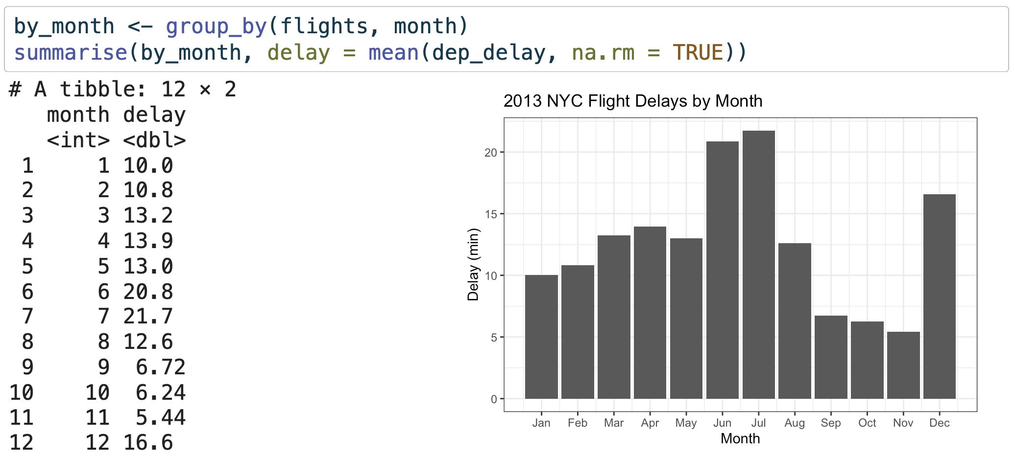

Multiple wrangles

by_dest <- group_by(flights, dest)

delay <- summarise(by_dest,
  count = n(),
  dist = mean(distance, na.rm = TRUE),
  delay = mean(arr_delay, na.rm = TRUE)
)

delay <- filter(delay, count > 20, dest != "HNL")

# It looks like delays increase with distance up to ~750 miles 
# and then decrease. Maybe as flights get longer there's more 
# ability to make up delays in the air?
ggplot(data = delay, mapping = aes(x = dist, y = delay)) +
  geom_point(aes(size = count), alpha = 1/3) +
  geom_smooth(se = FALSE)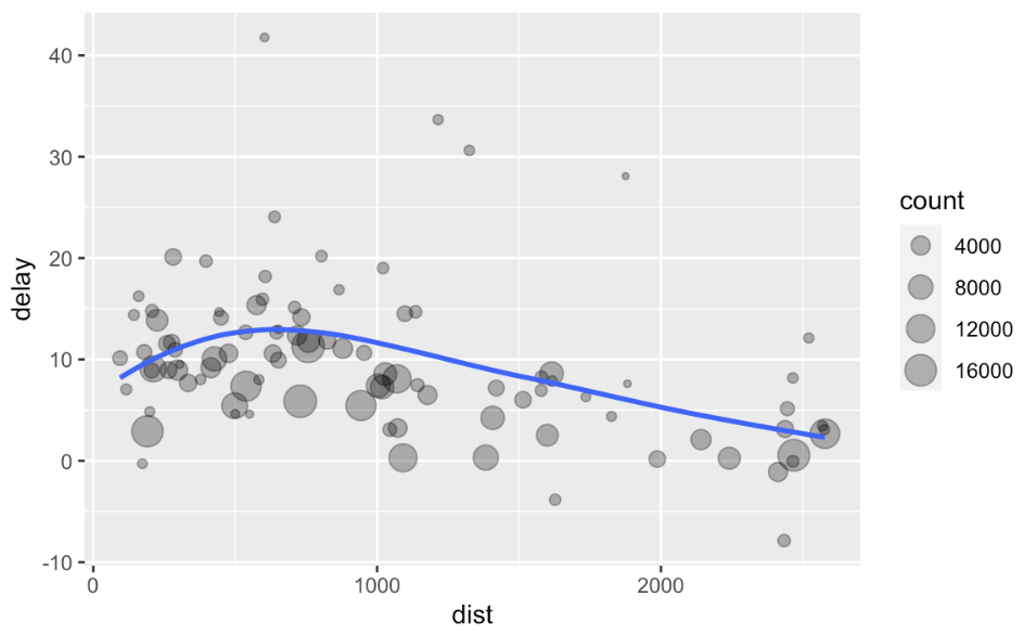

Multiple wrangles: `%>%`

delays <- flights %>% 
  group_by(dest) %>% 
  summarise(
    count = n(),
    dist = mean(distance, na.rm = TRUE),
    delay = mean(arr_delay, na.rm = TRUE)
  ) %>% 
  filter(count > 20, dest != "HNL")

ggplot(data = delays, mapping = aes(x = dist, y = delay)) +
  geom_point(aes(size = count), alpha = 1/3) +
  geom_smooth(se = FALSE)

5. Grouped summaries with `summarise()`

Useful summary functions

count(), min(), max(), quantile(), mean(), median(), sd()
read R for Data Science section 5.6.4 for a longer list

Summary of today

we learned five dplyr verbs for wrangling data:
- filter()
- arrange()
- select()
- mutate()
- summarise() (paired with group_by())

Data wrangling & visualization II — dplyr

Midterm & Final Exam Format

Data Transformation

The dplyr package

The dplyr package

The nycflights13 dataset

Install the nycflights13 package

Load required packages

flights

flights

flights

other variable types

dplyr basic verbs

1. filter()

1. Filter rows with filter()

1. Filter rows with filter()

1. Filter rows with filter()

1. Filter rows with filter()

1. Filter rows with filter()

Comparisons

Comparisons

Comparisons

Comparisons

Comparisons

Logical operators

Logical operators

Missing values

Missing values

2. arrange()

2. Arrange rows with arrange()

2. Arrange rows with arrange()

2. Arrange rows with arrange()

3. select()

3. Select columns with select()

3. Select columns with select()

3. Select columns with select()

3. Select columns with select()

4. mutate()

4. Add new variables with mutate()

4. Add new variables with mutate()

4. Add new variables with mutate()

4. Add new variables with mutate()

4. Add new variables with mutate()

4. Add new variables with mutate()

5. summarise()

5. Grouped summaries with summarise()

5. Grouped summaries with summarise()

5. Grouped summaries with summarise()

5. Grouped summaries with summarise()

5. Grouped summaries with summarise()

Multiple wrangles

Multiple wrangles: %>%

5. Grouped summaries with summarise()

Useful summary functions

Summary of today

The `dplyr` package

The `dplyr` package

The `nycflights13` dataset

Install the `nycflights13` package

`flights`

`flights`

`flights`

`dplyr` basic verbs

1. Filter rows with `filter()`

1. Filter rows with `filter()`

1. Filter rows with `filter()`

1. Filter rows with `filter()`

1. Filter rows with `filter()`

2. Arrange rows with `arrange()`

2. Arrange rows with `arrange()`

2. Arrange rows with `arrange()`

3. Select columns with `select()`

3. Select columns with `select()`

3. Select columns with `select()`

3. Select columns with `select()`

4. Add new variables with `mutate()`

4. Add new variables with `mutate()`

4. Add new variables with `mutate()`

4. Add new variables with `mutate()`

4. Add new variables with `mutate()`

4. Add new variables with `mutate()`

5. Grouped summaries with `summarise()`

5. Grouped summaries with `summarise()`

5. Grouped summaries with `summarise()`

5. Grouped summaries with `summarise()`

5. Grouped summaries with `summarise()`

Multiple wrangles: `%>%`

5. Grouped summaries with `summarise()`