Weekly homework assignments are comprised of two components: a Lab Component that your TA will guide you through in the weekly lab session, and a Home Component that you are to complete on your own. You must hand in both components. Both will count towards your grade.
Submit homework on OWL by 5:00 pm London ON time on the date shown in the Class Schedule.
Submit your homework assignment as a single RMarkdown file, using your last name and the homework assignment as a filename in the following format: gribble_n.Rmd where n is the homework assignment number.
Here is the R Markdown template file for this assignment: lastname_9.Rmd.
Lab Component
We will be using some sample data from Matthew Crump’s course, which is data from the following paper:
Rosenbaum D, Mama Y, Algom D (2017) Stand by Your Stroop: Standing Up Enhances Selective Attention and Cognitive Control. Psychol Sci 28:1864–1867
Available at: http://dx.doi.org/10.1177/0956797617721270
For this week’s lab we will be treating the data as a between-subjects design, in other words, we will be assuming that different participants provided observations in each of the 4 groups.
1. Load the data
library(tidyverse)
Warning: package 'lubridate' was built under R version 4.3.1
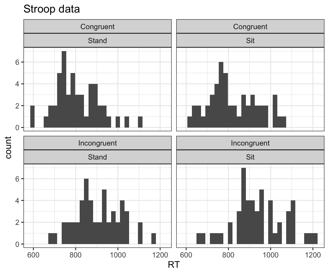
Plot some histograms showing each group in the 2x2 design. Use the facet_wrap() function to create a 2x2 grid of plots. Here is an example (but it is only an example):
Compute means and standard errors for each group. Use group_by() and summarise() to create a new data frame with the means, standard errors, and n for each group.
# A tibble: 4 × 5
# Groups:   Congruency [2]
  Congruency  Posture meanRT    se     n
  <fct>       <fct>    <dbl> <dbl> <int>
1 Congruent   Stand     808.  14.9    50
2 Congruent   Sit       822.  16.6    50
3 Incongruent Stand     904.  15.3    50
4 Incongruent Sit       941.  17.9    50
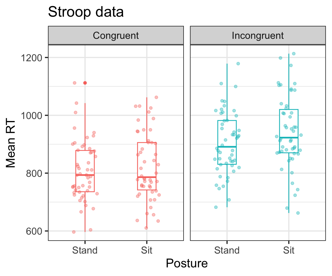
Create a plot of your choosing showing mean RTs for each group with error bars indicating standard errors, and overlay the raw data points using geom_jitter(). Here is an example (but it is only an example):
3. Compute the ANOVA
Use aov() to compute a 2x2 factorial ANOVA for the data. Use summary() to print the results.
Report the results of the ANOVA. In particular, report the results of the two main effects tests and the interaction test. What do these results tell you about the effect of congruency and posture on RT? Use marginal means to describe the effects. Don’t worry about doing post-hoc statistical tests yet (we will do that next week), just interpret the means.
4. Check assumptions
4.1. Normality
Check the normality assumption by (a) a Q-Q plot of the residuals of the ANOVA model, and (b) using the Shapiro test on the residuals. Report and interpret the results.
    Shapiro-Wilk normality test

data:  residuals(my.anova)
W = 0.98681, p-value = 0.05967
4.2 Homogeneity of variance
Check the homogeneity of variance assumption using leveneTest() from the car package. Report and interpret the results.
Levene's Test for Homogeneity of Variance (center = median)
       Df F value Pr(>F)
group   3  0.5212 0.6682
      196
Home Component
1. Load the data
From a textbook by Maxwell & Delaney—A clinical psychologist is interested in three types of therapy for modifying snake phobia. However, she does not believe that one type is necessarily best for everyone; instead, the best type may depend on degree (i.e., severity) of phobia. Undergraduate students enrolled in an introductory psychology course are given the Fear Schedule Survey (FSS) to screen out subjects showing no fear of snakes. Those displaying some degree of phobia are classified as either mildly, moderately, or severely phobic on the basis of the FSS. One third of subjects within each level of severity are then assigned to a treatment condition: systematic desensitization, implosive therapy, or insight therapy. Thus this is a 2-way between subjects design, with 3 levels in each of the two factors. So this is a 3x3 between subjects design.
The following data are obtained, using the Behavioral Avoidance Test as the dependent variable (higher scores are better):
Compute the mean, standard error, and sample size for each of the nine groups. Use group_by() and summarise() to create a new data frame with the means, standard errors, and n for each group.
3. Visualize the data
Generate a plot of your choosing showing mean BAT for each group with error bars indicating standard errors, and overlay the raw data points using geom_jitter().
4. Compute the ANOVA
Use aov() to compute a 3x3 factorial ANOVA for the data. Use summary() to print the results.
Report the results of the ANOVA. In particular, report the results of the two main effects tests and the interaction test. What do these results tell you about the effect of Treatment and Phobia on BAT? Don’t worry about doing post-hoc statistical tests yet (we will do that next week), just interpret the means.
5. Check assumptions
5.1. Normality
Check the normality assumption by (a) a Q-Q plot of the residuals of the ANOVA model, and (b) using the Shapiro test on the residuals. Report and interpret the results.
5.2 Homogeneity of variance
Check the homogeneity of variance assumption using leveneTest() from the car package. Report and interpret the results.