Weekly homework assignments are comprised of two components: a Lab Component that your TA will guide you through in the weekly lab session, and a Home Component that you are to complete on your own. You must hand in both components. Both will count towards your grade.
Submit homework on OWL by 5:00 pm London ON time on the date shown in the Class Schedule.
Submit your homework assignment as a single RMarkdown file, using your last name and the homework assignment as a filename in the following format: gribble_n.Rmd where n is the homework assignment number.
Here is the R Markdown template file for this assignment: lastname_7.Rmd.
Lab Component
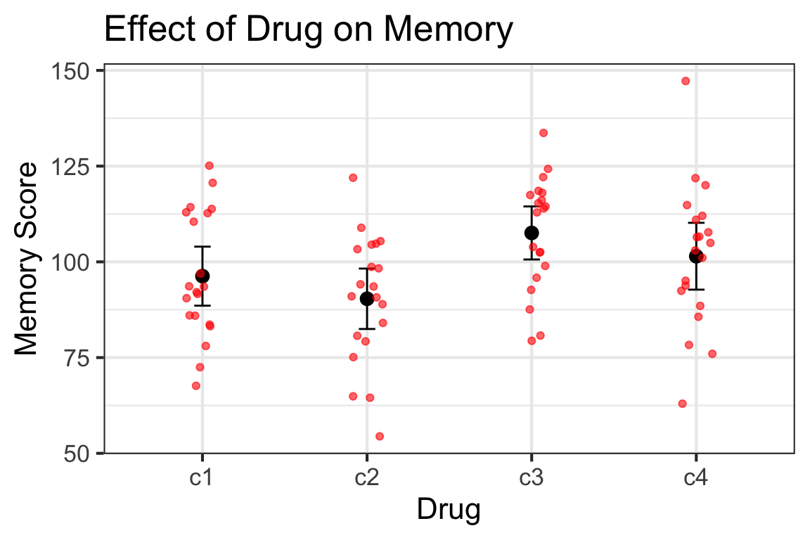
We will look at a dataset (from https://pnb.mcmaster.ca/bennett/psy710) in which a dependent variable called “score” was measured in 4 groups of participants. Let’s pretend that score is each participant’s score on a memory test and condition is four different drugs they ingested prior to the memory test. We want to know if the drugs affect memory.
Generate a plot of the data with the groups on the x-axis and the visual acuity score on the y-axis. Use the geom_jitter() function to add some jitter to the points. Your plot doesn’t have to look exactly like this one but this gives you an example. Here I plot the mean of each group (a filled black circle) and error bars representing the 95 % confidence interval of the mean. The red points are the individual observations, jittered horizontally to avoid overplotting.
4. Fit the ANOVA linear model to the data
Fit the ANOVA linear model to the data. Use the aov() function. Print the summary of the model.
            Df Sum Sq Mean Sq F value Pr(>F)
condition    3   3226  1075.2   3.832  0.013 *
Residuals   76  21328   280.6
---
Signif. codes:  0 '***' 0.001 '**' 0.01 '*' 0.05 '.' 0.1 ' ' 1
Home Component
5. Test the normality assumption
Test the normality assumption for ANOVA. Produce at least one graphical visualization that assesses normality, and interpret it. Also conduct a statistical test to assess the normality assumption. What is the null hypothesis for this test? What does the p-value mean? Interpret the results of the test. Finally declare whether or not you think the normality assumption is met.
6. Test the homogeneity of variance assumption
Test the homogeneity of variance assumption for ANOVA. Conduct a statistical test to assess the homogeneity of variance assumption. What is the null hypothesis for this test? What does the p-value mean? Interpret the results of the test. Finally declare whether or not you think the homogeneity of variance assumption is met.
7. Interpret the results of the ANOVA
With reference to the summary() of the aov() object, interpret the results of the ANOVA. What is the effect of the independent variable on the dependent variable? What is the p-value for the F-test? What does this p-value mean?
Next week we will learn how to do statistical follow-up tests to determine which groups are different from each other. But for now, in everyday language, describe what you think the effect of the drugs on memory might be. For example does each drug affect memory differently? Is the one drug that stands out? Are there two drugs that stand out from the other two? etc.
8. Effect size
Install the package effectsize and load it into R.
Compute eta-squared for the ANOVA model, using the eta_squared() function. Interpret the results.