Weekly homework assignments are comprised of two components: a Lab Component that your TA will guide you through in the weekly lab session, and a Home Component that you are to complete on your own. You must hand in both components. Both will count towards your grade.
Submit homework on OWL by 5:00 pm London ON time on the date shown in the Class Schedule.
Submit your homework assignment as a single RMarkdown file, using your last name and the homework assignment as a filename in the following format: gribble_n.Rmd where n is the homework assignment number.
Here is the R Markdown template file for this assignment: lastname_6.Rmd.
The dataset contains 100 observations of 4 variables:
dan.sleep: how much sleep Daniella had that night
baby.sleep: how much sleep Daniella’s baby had that night
dan.grump: a grumpiness index of how grumpy Daniella was that day
day: the day
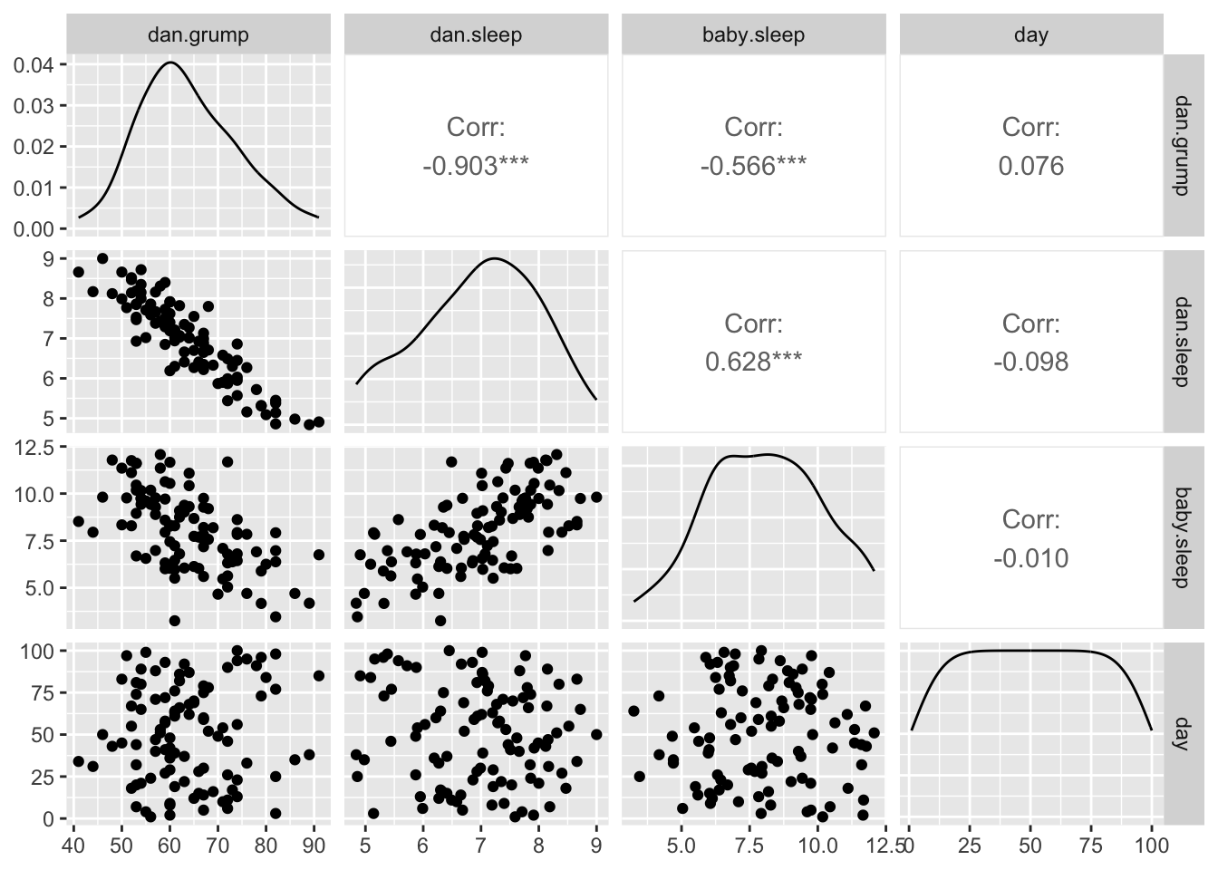
2. Examine correlations
Use ggpairs() from the GGally package to visualize the correlations between each pair of variables in the dataset. Describe what you see and what it means.
3. Model Daniella’s grumpiness
Fit a “full model” mod.full in which you predict dan.grump based on the other three variables: dan.sleep, baby.sleep, and day. Show the model summary() and describe and interpret:
the overall Multiple R-squared
the overall p-value for the model as a whole
the model coefficients (called “Estimate” in the summary() output)
Call:
lm(formula = dan.grump ~ dan.sleep + baby.sleep + day, data = parenthood)

Residuals:
    Min      1Q  Median      3Q     Max
-10.906  -2.284  -0.295   2.652  11.880

Coefficients:
              Estimate Std. Error t value Pr(>|t|)
(Intercept) 126.278707   3.242492  38.945   <2e-16 ***
dan.sleep    -8.969319   0.560007 -16.016   <2e-16 ***
baby.sleep    0.015747   0.272955   0.058    0.954
day          -0.004403   0.015262  -0.288    0.774
---
Signif. codes:  0 '***' 0.001 '**' 0.01 '*' 0.05 '.' 0.1 ' ' 1

Residual standard error: 4.375 on 96 degrees of freedom
Multiple R-squared:  0.8163,    Adjusted R-squared:  0.8105
F-statistic: 142.2 on 3 and 96 DF,  p-value: < 2.2e-16
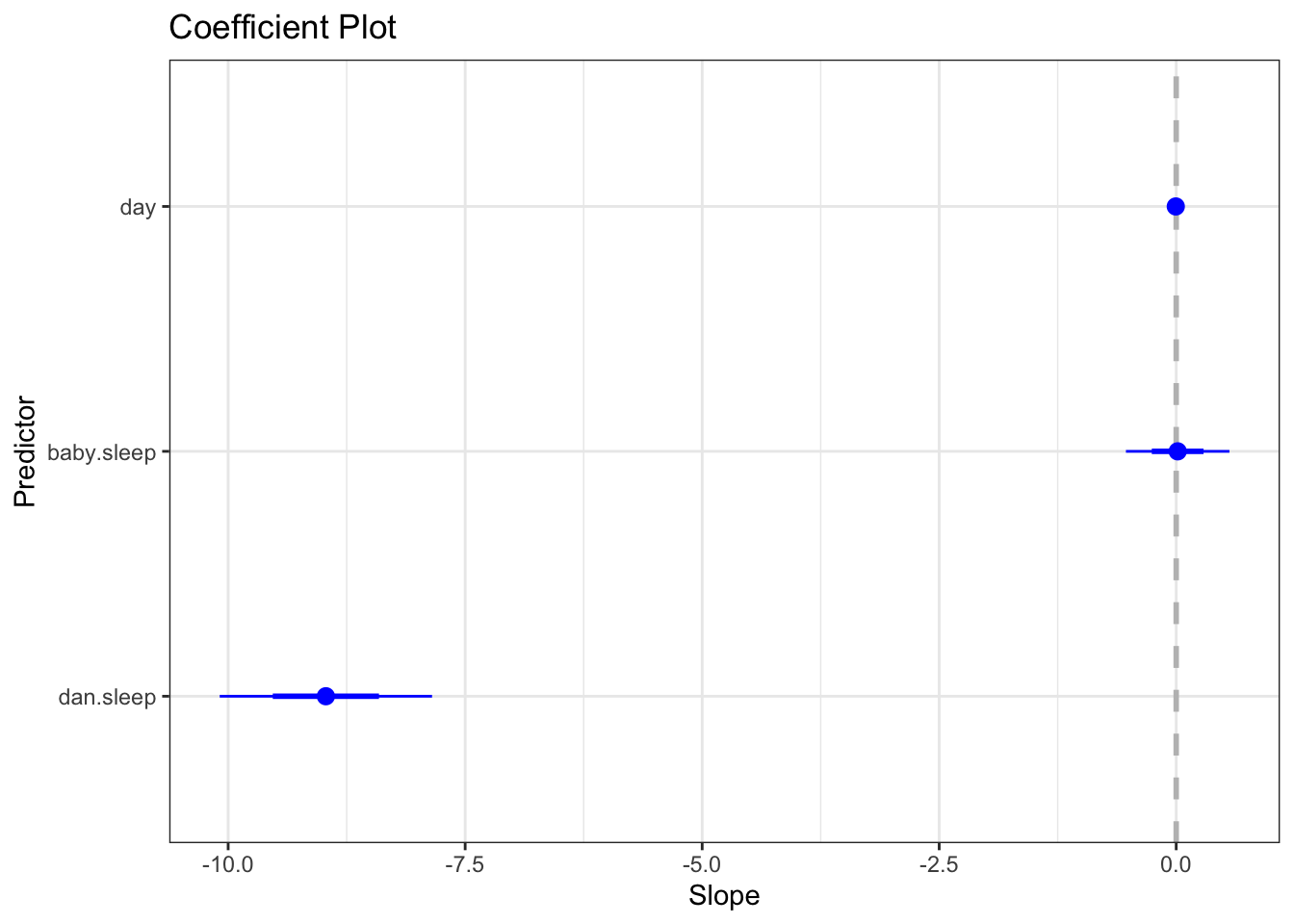
4. Plot model coefficients
Plot the slopes (model coefficients) relative to zero to better visualize them.
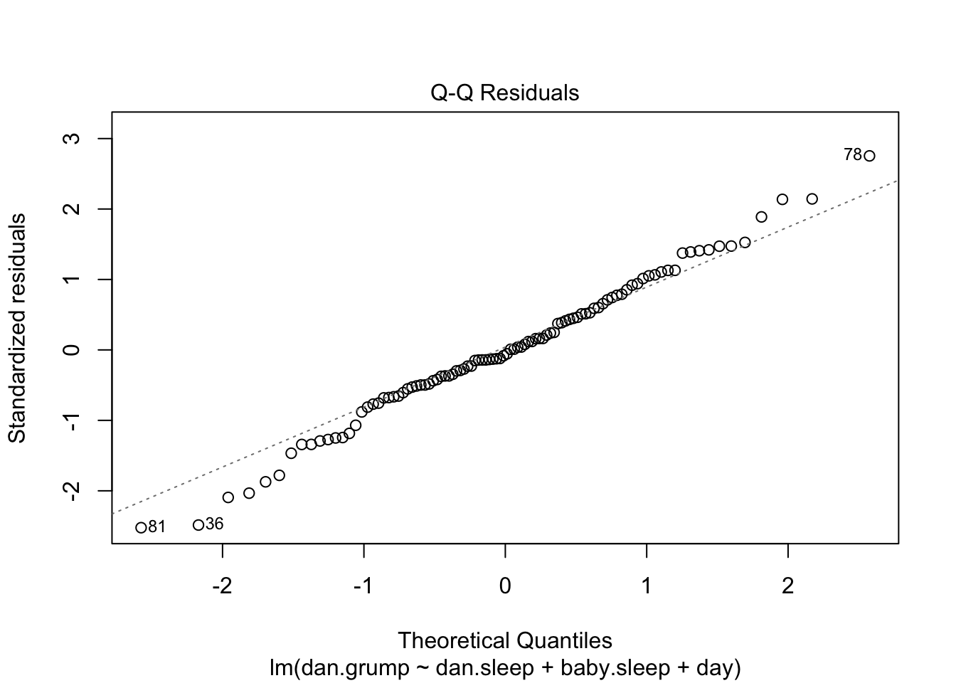
5. Check assumptions
Check normality by producing a Q-Q plot. Interpet.
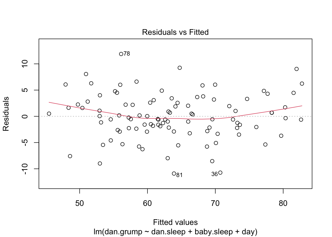
Check linearity by producing a plot of residuals and interpret.
Check for normality using shapiro.test(). Pass shapiro.test() the residuals of your model using residuals()
    Shapiro-Wilk normality test

data:  residuals(mod.full)
W = 0.9922, p-value = 0.8352
Check for heteroscedasticity by reference to the residual plot above. Interpet.
Check for heteroscedasticity using ncvTest() from the car package and interpet.
Non-constant Variance Score Test
Variance formula: ~ fitted.values
Chisquare = 0.118263, Df = 1, p = 0.73093
6. Refine the model
Use the step() procedure with the direction=both() option to test if you can refine the model further by eliminating any variables from the full model that don’t account for unique portions of variance in dan.grump. Start the procedure from the full model.
Describe the output of the step() procedure and what it means. Describe the refined model and how it differs (if it differs) from the full model, and why.
Start:  AIC=299.08
dan.grump ~ dan.sleep + baby.sleep + day

             Df Sum of Sq    RSS    AIC
- baby.sleep  1       0.1 1837.2 297.08
- day         1       1.6 1838.7 297.16
<none>                    1837.1 299.08
- dan.sleep   1    4909.0 6746.1 427.15

Step:  AIC=297.08
dan.grump ~ dan.sleep + day

             Df Sum of Sq    RSS    AIC
- day         1       1.6 1838.7 295.17
<none>                    1837.2 297.08
+ baby.sleep  1       0.1 1837.1 299.08
- dan.sleep   1    8103.0 9940.1 463.92

Step:  AIC=295.17
dan.grump ~ dan.sleep

             Df Sum of Sq    RSS    AIC
<none>                    1838.7 295.17
+ day         1       1.6 1837.2 297.08
+ baby.sleep  1       0.0 1838.7 297.16
- dan.sleep   1    8159.9 9998.6 462.50
Call:
lm(formula = dan.grump ~ dan.sleep, data = parenthood)

Residuals:
    Min      1Q  Median      3Q     Max
-11.025  -2.213  -0.399   2.681  11.750

Coefficients:
            Estimate Std. Error t value Pr(>|t|)
(Intercept) 125.9563     3.0161   41.76   <2e-16 ***
dan.sleep    -8.9368     0.4285  -20.85   <2e-16 ***
---
Signif. codes:  0 '***' 0.001 '**' 0.01 '*' 0.05 '.' 0.1 ' ' 1

Residual standard error: 4.332 on 98 degrees of freedom
Multiple R-squared:  0.8161,    Adjusted R-squared:  0.8142
F-statistic: 434.9 on 1 and 98 DF,  p-value: < 2.2e-16
7. Predict
Using your refined model, predict how grumpy Daniella will be (i.e. the grumpiness index dan.grump) on a future day if she obtains 6.0 hours of sleep.
       1
72.33576
With reference to the model coefficient(s), how much does the dan.grump index change and in what direction, for every additional hour of sleep?
Home Component
You are being considered for a position as the new coach of a basketball team. You just finished a meeting with the owners, who are interested in replacing the existing coach because the team’s performance has been going downhill. The owners of the team have attributed this downward trend to poor recruitment of new players, who have been poor performers. The owners tell you that their analysis of the data from the previous seasons indicates that one particularly weak area has been “field goals” (when a player attempts to score a basket from the 3-point line or beyond). The team’s players, in particular the new recruits, tend to be poor at field goals. The problem is, as the owners tell you, that data are not available on field goal percentages, for players who are candidate recruits; so when it comes time to recruit new players there is no easy way to pick new recruits who are good field goal shooters. The owners tell you that they have been collecting data for years and years on the new recruits and their field goal percentages, and a series of other measures that are available for the new potential recruits as well. She suggests that “if you can use the historical data to be able to predict who among the potential new recruits will be the best field goal shooters, you are hired!”
In the file called https://www.gribblelab.org/2812/data/bball.csv you will find historical data on 105 previous recruits. The variables are:
GAMES : # games played in previous season
PPM : average points scored per minute
MPG : average minutes played per game
HGT : height of player (centimetres)
FGP : field-goal percentage (% successful shots from 3-point line)
AGE : age of player (years)
FTP : percentage of successful penalty free throws
In the file https://www.gribblelab.org/2812/data/bball2.csv you will find data on 5 potential new recruits.
8. Develop a model
Use multiple regression to develop a refined model based on the data in bball.csv that will allow you to predict the field goal percentages for the 5 new recruits. Use summary() to show the refined model that you propose. Show your work. Explain in words the process you used to arrive at your final model. Check linearity, normality and homoscedasticity assumptions (of the full model, before you refine the model). Describe the influence each variable in your refined model has on predicting FGP, with reference to the coefficients (slope parameters).
9. Propose a player
Based on your model, which player will you suggest to the owners that they hire? Explain your decision.
10. Precision
Given your model, what is the precision (in units of FGP) with which you can predict field goal percentage?
11. Age & Height
After giving them your recommendation and explaining your model, the owners ask you “does the player’s age have anything to do with this?” Answer with reference to your model.
“What about the player’s height? Would I be better off taking on taller players?” Answer with reference to your model.
According to the multiple regression model you developed, how many more (or fewer) field goals would a player score if they were 3 inches taller? Explain with reference to your model. Assume 2.54 centimetres per inch.