install.packages("palmerpenguins")Homework 2
Psychology 2812B FW22
Weekly homework assignments are comprised of two components: a Lab Component that your TA will guide you through in the weekly lab session, and a Home Component that you are to complete on your own. You must hand in both components. Both will count towards your grade.
Submit homework on OWL by 5:00 pm London ON time on the date shown in the Class Schedule.
Submit your homework assignment as a single RMarkdown file, using your last name and the homework assignment as a filename in the following format: gribble_n.Rmd where n is the homework assignment number.
Here is the R Markdown template file for this assignment: lastname_2.Rmd.
Lab Component
1. Install/load the penguins dataset
In RStudio install the palmerpenguins dataset (you will only have to do this once)
Load the palmerpenguins dataset into memory (to access the penguins dataset you will have to do this each time you start RStudio)
library("palmerpenguins")Have a look at the first few rows of the data table
penguins# A tibble: 344 × 8
species island bill_length_mm bill_depth_mm flipper_length_mm body_mass_g
<fct> <fct> <dbl> <dbl> <int> <int>
1 Adelie Torgersen 39.1 18.7 181 3750
2 Adelie Torgersen 39.5 17.4 186 3800
3 Adelie Torgersen 40.3 18 195 3250
4 Adelie Torgersen NA NA NA NA
5 Adelie Torgersen 36.7 19.3 193 3450
6 Adelie Torgersen 39.3 20.6 190 3650
7 Adelie Torgersen 38.9 17.8 181 3625
8 Adelie Torgersen 39.2 19.6 195 4675
9 Adelie Torgersen 34.1 18.1 193 3475
10 Adelie Torgersen 42 20.2 190 4250
# ℹ 334 more rows
# ℹ 2 more variables: sex <fct>, year <int>Also have a read through the documentation for the dataset by typing ?penguins in RStudio (it will show the documentation in the Help panel).
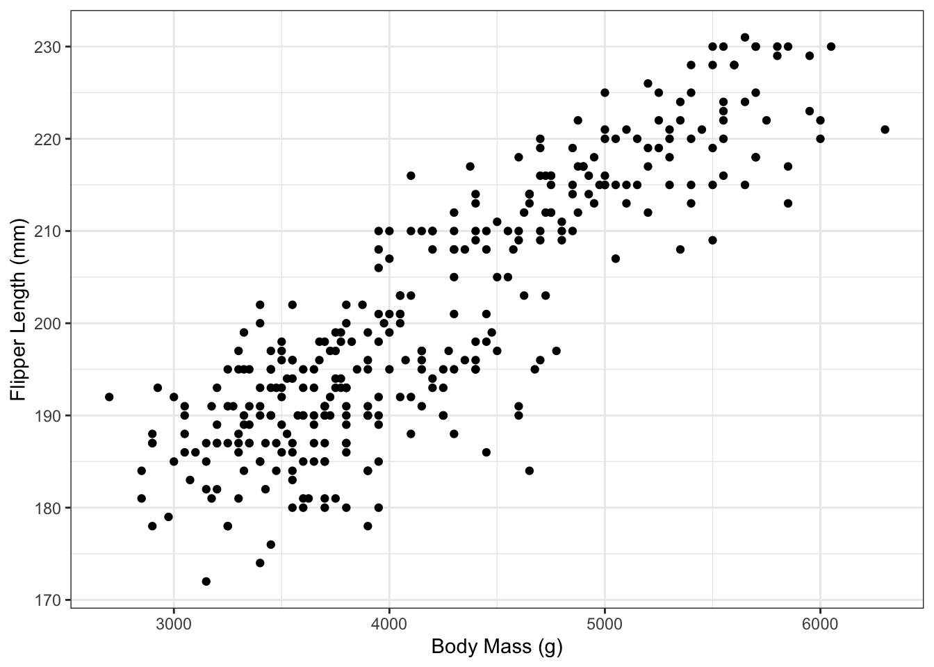
2. Scatterplot
Make a plot of flipper length as a function of body mass. Use the theme_bw() theme. Make the labels on the x-axis and y-axis more human friendly than the default column names in the data tibble—use the labs() instruction with x=" " and y=" " arguments to specify labels for the x- and y-axes.
don’t forget to load the tidyverse into memory each time you startup RStudio, using library(tidyverse)
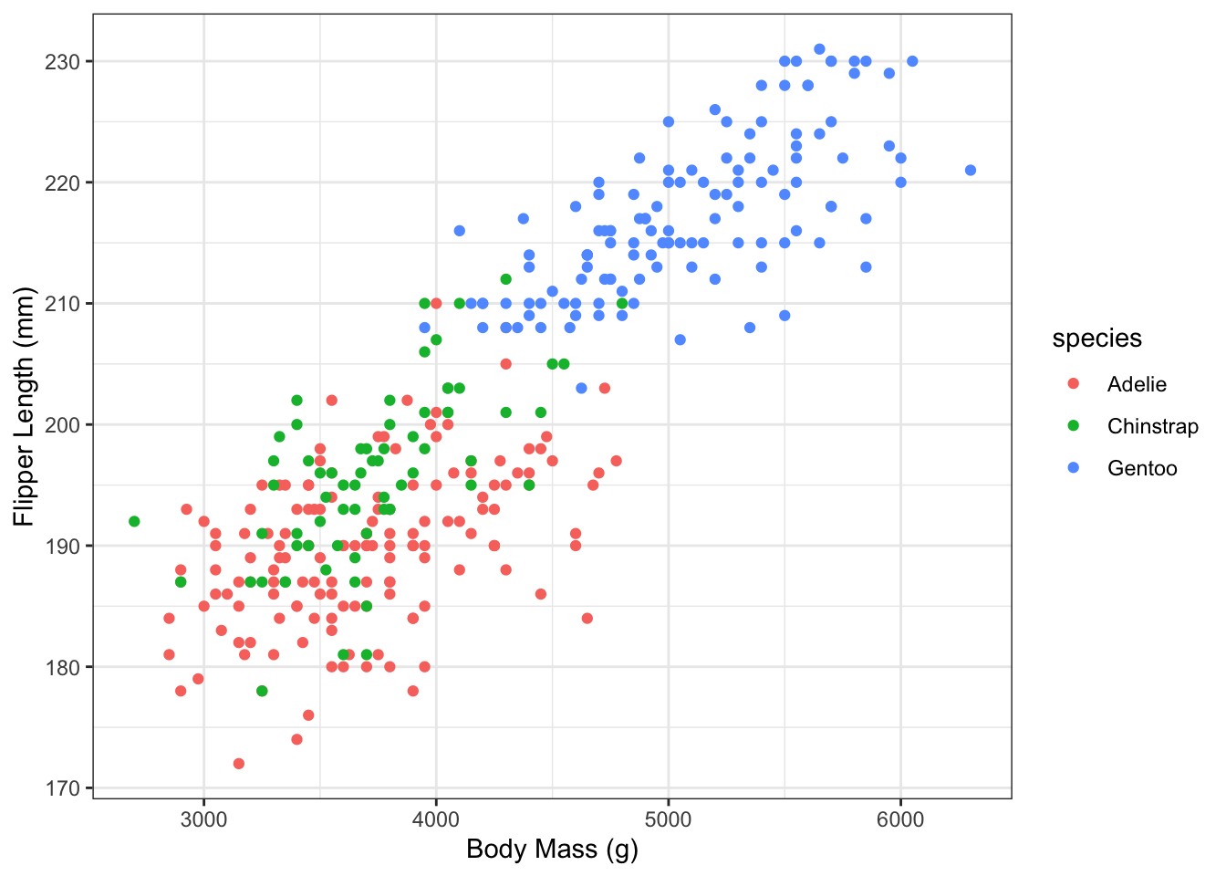
3. Colour by Species
Re-plot using different colours to code the three different pengiun species.
Home Component
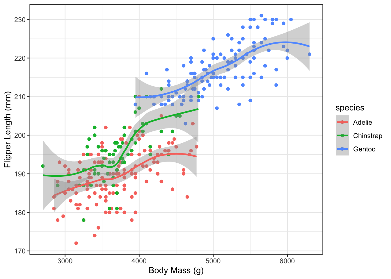
4. Smoothing lines
Re-plot and add a smoother line using geom_smooth()
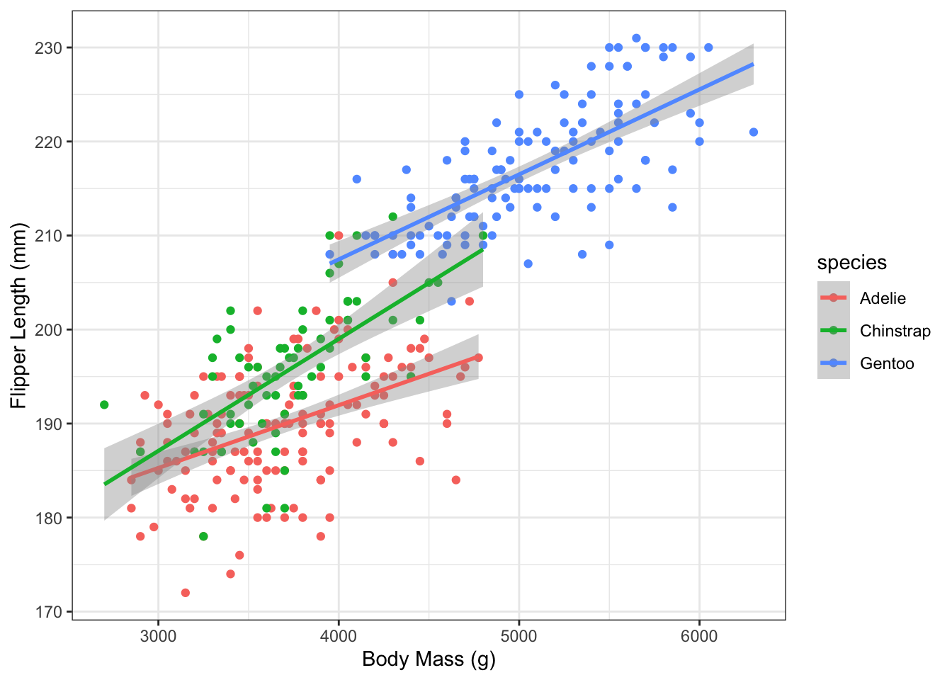
5. Linear fit
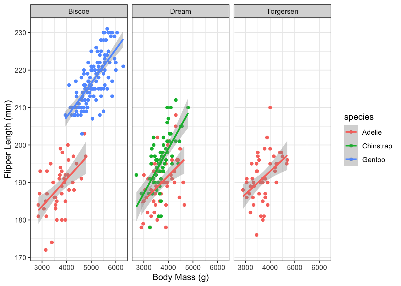
Re-plot using a linear fit smoothing line. Hint: the geom_smooth() function takes a method argument and if you give it method = "lm" it will use a linear fit.
6. Facet by island
Re-plot using different facets for each island, with the facets arranged along 1 row. Hint: use the facet_wrap() function with nrow = 1.
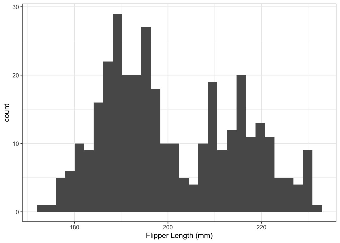
7. Histogram
Generate a histogram of flipper lengths. Hint: there is a geometric object called geom_histogram(). Set the x label to Flipper Length (mm) (hint: there is a layer instruction for labels called labs()):
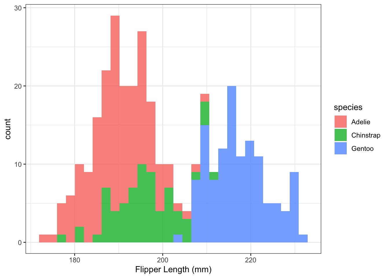
8. Colour by species
Replot the histogram above but specify that the fill color of the bars should be coded by species (fill = species).
Hint: this is an aesthetic mapping (a mapping of variables in the dataset onto different aesthetic qualities of the plot) and so you will have to put the fill = species instruction within an aes() function call. Where should this aesthetic mapping live? Play around with different possibilities. Can you simply add fill = species to an aes() call that lives within the call to ggplot()? Could you instead add a new aes() call within the geom_histogram() instruction? Decide on one solution and write a sentence explaining your choice.
Specify the alpha transparency of the bars to be alpha = 0.8 so that you can see the different colors overlapping.
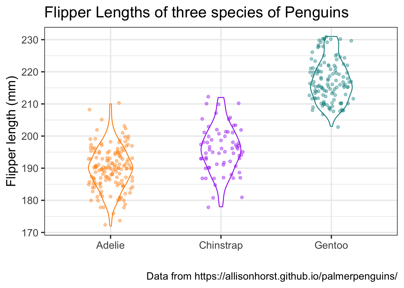
9. Boxplot
Here is some code that layers a box plot of flipper lengths across species together with jittered points of each penguin. Study each component and play with it to understand how it works.
ggplot(data = penguins,
       mapping = aes(x = species, y = flipper_length_mm)) +
  geom_boxplot(aes(color = species), width = 0.3, show.legend = FALSE) +
  geom_jitter(aes(color = species), alpha = 0.4, show.legend = FALSE, width = 0.2) +
  scale_color_manual(values = c("darkorange","purple","cyan4")) +
  labs(x = "",
       y = "Flipper length (mm)") +
theme_bw() 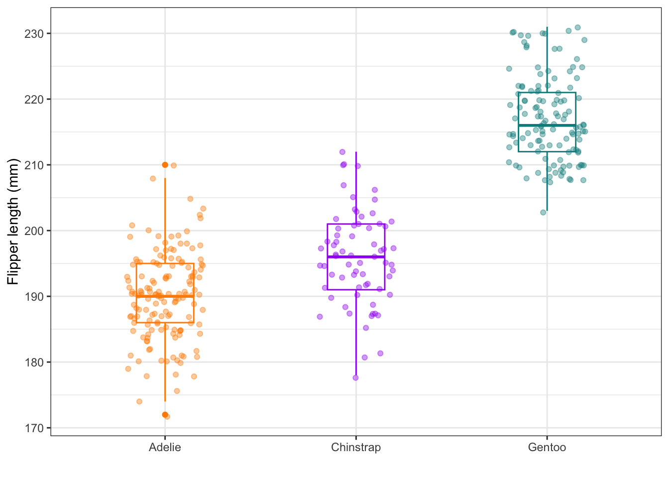
Re-plot this figure using a violin plot instead of a boxplot. Hint: there is a geom object for violin plots. Set the width of the violins to be equal to 0.4. Also add a title and a caption to the plot. Also change the base_size of the fonts to 16.
Note: since we are using a random jitter for the points, the location of the points on your plot may not look exactly like they do on mine. That is ok.
Help!
how to look things up when you don’t know what do to?
- check the assigned readings (the R for Data Science online book has a search box)
- check the ggplot2 documentation, it also has a search box
- when you find the correct command, take a moment to try to understand how/why it works and how it fits with the ggplot2 concept of the layered grammar of graphics