%% Generate a signal
t = 0:.001:0.5;           % 0.5 seconds sampled every 1 ms (1000 Hz sampling rate)
y1 = sin(2*pi*125 * t);   % pure sinusoid at 125 Hz
y2 = sin(2*pi*30 * t);    % pure sinusoid at 30 Hz
y3 = sin(2*pi*300 * t);   % pure sinusoid at 300 Hz
y = y1 + (0.8*y2) + (0.9*y3);
figure;
subplot(2,1,1)
plot(t,y,'-'); xlabel('TIME (sec)'); ylabel('SIGNAL');

%% perform an FFT of the signal and plot the spectrum
%[f, m, p] = fft_plus (y, 1000);
[m,f] = pwelch(y, [], [], [], 1000);
subplot(2,1,2)
plot(f,m,'.-'); xlabel('Frequency (Hz)'); ylabel('Magnitude')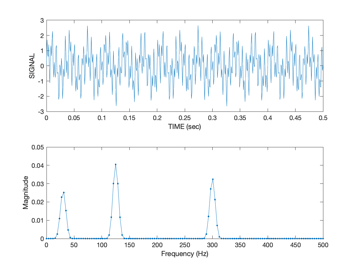

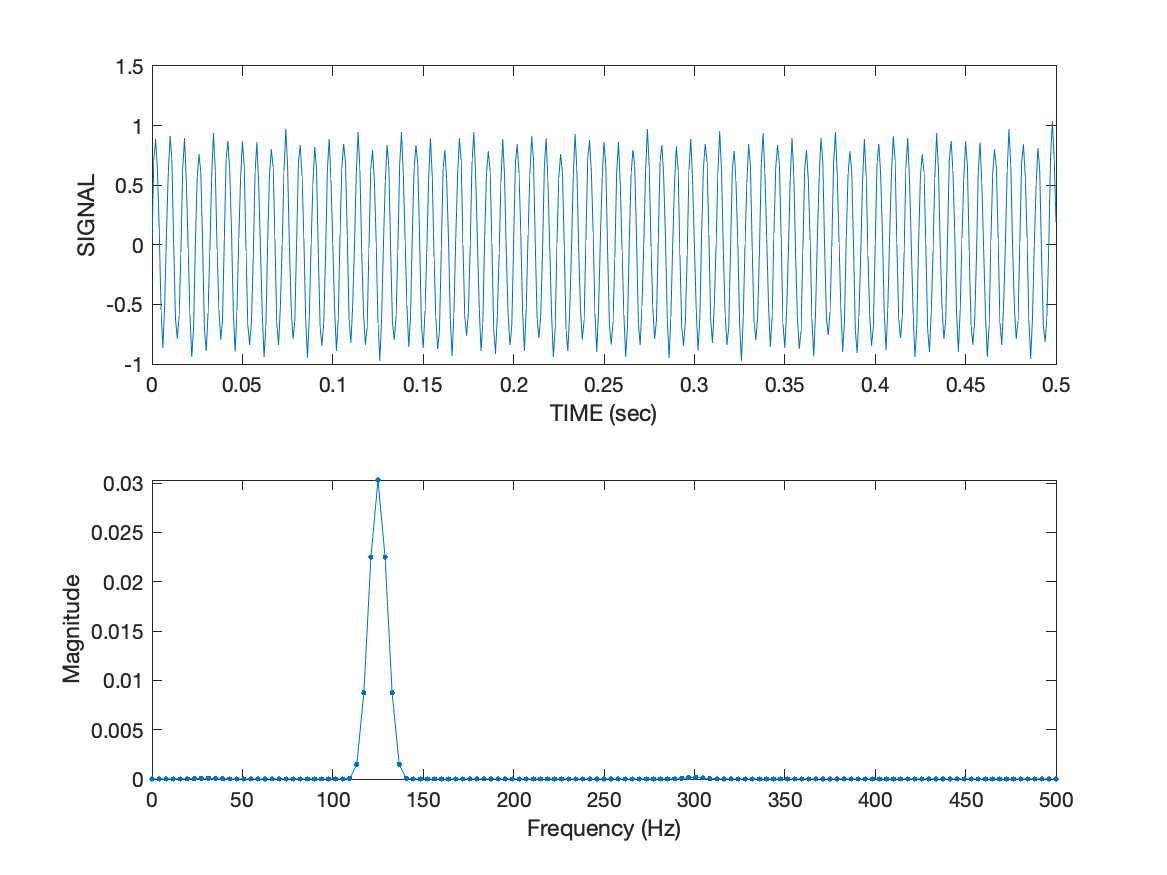
%% lowpass the signal to remove the 300 Hz component
y_f = PLGlowpass(y,1000,200);
%[f_f, m_f, p_f] = fft_plus (y_f, 1000);
[m_f,f_f] = pwelch(y_f, [], [], [], 1000);
figure;
subplot(2,1,1)
plot(t,y_f,'-'); xlabel('TIME (sec)'); ylabel('SIGNAL');
subplot(2,1,2)
plot(f_f,m_f,'.-'); xlabel('Frequency (Hz)'); ylabel('Magnitude')

%% highpass the signal to remove the 30 Hz component
y_f = PLGhighpass(y_f,1000,60);
%[f_f, m_f, p_f] = fft_plus (y_f, 1000);
[m_f,f_f] = pwelch(y_f, [], [], [], 1000);
figure;
subplot(2,1,1)
plot(t,y_f,'-'); xlabel('TIME (sec)'); ylabel('SIGNAL');
subplot(2,1,2)
plot(f_f,m_f,'.-'); xlabel('Frequency (Hz)'); ylabel('Magnitude')