Scientific Computing (Psychology 9040a)

In this chapter we will use a model of voltage-gated ion channels in a single neuron to simulate action potentials. The model is based on the work by Hodgkin & Huxley in the 1940s and 1950s. A good reference to refresh your memory about how ion channels in a neuron work is the Kandel, Schwartz & Jessel book “Principles of Neural Science”.

Introduction

To model the action potential we will use an article by Ekeberg et al. (1991) published in Biological Cybernetics (see citation above). When reading the article you can focus on the first three pages (up to paragraph 2.3) and try to find answers to the following questions:

Before we begin coding up the model, it may be useful to remind you of a fundamental law of electricity, one that relates electrical potential \(V\) to electric current \(I\) and resistance \(R\) (or conductance \(G\), the reciprocal of resistance). This of course is known as Ohm’s law:

Our goal here is to code up a dynamical model of the membrane’s electric circuit including two types of ion channels: sodium and potassium channels. We will use this model to better understand the process underlying the origin of an action potential.

The Neuron Model

The Figure below, adapted from Ekeberg et al., 1991, schematically illustrates the model of a neuron. In panel A we see a soma, and multiple dendrites. Each of these can be modelled by an electrical “compartment” (Panel B) and the passive interactions between them can be modelled as a pretty standard electrical circuit (see Biological Neuron Model for more details about compartmental models of neurons). In panel C, we see an expanded model of the Soma from panel A. Here, a number of active ion channels are included in the model of the soma.

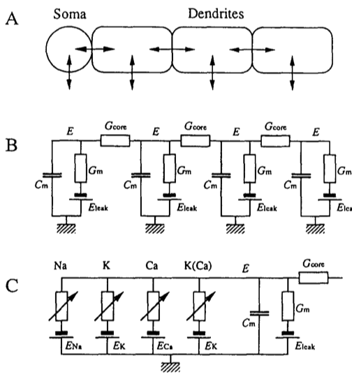
For our purposes here, we will focus on the soma, and we will not include any additional dendrites in our implementation of the model. Thus essentially we will be modelling what appears in panel C, and at that, only a subset.

In panel C we see that the soma can be modelled as an electrical circuit with a sodium ion channel (Na), a potassium ion channel (K), a calcium ion channel (Ca), and a calcium-dependent potassium channel (K(Ca)). What we will be concerned with simulating, ultimately, is the intracellular potential E.

Passive Properties

Equation (1) of Ekeberg is a differential equation describing the relation between the time derivative of the membrane potential \(E\) as a function of the passive leak current through the membrane, and the current through the ion channels. Note that Ekeberg uses \(E\) instead of the typical \(V\) symbol to represent electrical potential.

\[\frac{dE}{dt} = \frac{(E_{leak}-E)G_{m} + \sum{\left(E_{comp}-E\right)}G_{core} + I_{channels}}{C_{m}}\]

Don’t panic, it’s not actually that complicated. What this equation is saying is that the rate of change of electrical potential across the current (the left hand side of the equation, \(\frac{dE}{dt}\)) is equal to the sum of a bunch of other terms, divided by membrane capacitance \(C_{m}\) (the right hand side of the equation). Recall from basic physics that capacitance is a measure of the ability of something to store an electrical charge.

The “bunch of other things” is a sum of three things, actually, (from left to right): a passive leakage current, plus a term characterizing the electrical coupling of different compartments, plus the currents of the various ion channels. Since we are not going to be modelling dendrites here, we can ignore the middle term on the right hand side of the equation \(\sum{\left(E_{comp}-E\right)}G_{core}\) which represents the sum of currents from adjacent compartments (we have none).

We are also going to include in our model an external current \(I_{ext}\). This can essentially represent the sum of currents coming in from the dendrites (which we are not explicitly modelling). It can also represent external current injected in a patch-clamp experiment. This is what we as experimenters can manipulate, for example, to see how neuron spiking behaviour changes. So what we will actually be working with is this:

What we need to do now is unpack the \(I_{channels}\) term representing the currents from all of the ion channels in the model. Initially we will only be including two, the potassium channel (K) and the sodium channel (Na).

Sodium Channels (Na)

The current through sodium channels that enter the soma are represented by equation (2) in Ekeberg et al. (1991):

where \(m\) is the activation of the sodium channel and \(h\) is the inactivation of the sodium channel, and the other terms are constant parameters: \(E_{Na}\) is the reversal potential, \(G_{Na}\) is the maximum sodium conductance throught the membrane, and \(E_{soma}\) is the membrane potential of the soma.

The activation \(m\) of the sodium channels is described by the differential equation (3) in Ekeberg et al. (1991):

where \(\alpha_{m}\) represents the rate at which the channel switches from a closed to an open state, and \(\beta_{m}\) is rate for the reverse. These two parameters \(\alpha\) and \(\beta\) depend on the membrane potential in the soma. In other words the sodium channel is voltage-gated. Equation (4) in Ekeberg et al. (1991) gives these relationships:

\[\begin{aligned} \alpha_{m} &= &\frac{A(E_{soma}-B)}{1-e^{(B-E_{soma})/C}}\\ \beta_{m} &= &\frac{A(B-E_{soma})}{1-e^{(E_{soma}-B)/C}}\end{aligned}\]

A tricky bit in the Ekeberg et al. (1991) paper is that the \(A\), \(B\) and \(C\) parameters above are different for \(\alpha\) and \(\beta\) even though there is no difference in the symbols used in the equations.

The inactivation of the sodium channels is described by a similar set of equations: a differential equation giving the rate of change of the sodium channel deactivation, from Ekeberg et al. (1991) equation (5):

and equations specifying how \(\alpha_{h}\) and \(\beta_{h}\) are voltage-dependent, given in Ekeberg et al. (1991) equation (6):

\[\begin{aligned} \alpha_{h} &= &\frac{A(B-E_{soma})}{1-e^{(E_{soma}-B)/C}}\\ \beta_{h} &= &\frac{A}{1-e^{(B-E_{soma})/C}}\end{aligned}\]

Note again that although the terms \(A\), \(B\) and \(C\) are different for \(\alpha_{h}\) and \(\beta_{h}\) even though they are represented by the same symbols in the equations.

So in summary, for the sodium channels, we have two state variables: \((m,h)\) representing the activation (\(m\)) and deactivation (\(h\)) of the sodium channels. We have a differential equation for each, describing how the rate of change (the first derivative) of these states can be calculated: Ekeberg equations (3) and (5). Those differential equations involve parameters \((\alpha,\beta)\), one set for \(m\) and a second set for \(h\). Those \((\alpha,\beta)\) parameters are computed from Ekeberg equations (4) (for \(m\)) and (6) (for \(h\)). Those equations involve parameters \((A,B,C)\) that have parameter values specific to \(\alpha\) and \(\beta\) and \(m\) and \(h\) (see Table 1 of Ekeberg et al., 1991).

Potassium Channels (K)

The potassium channels are represented in a similar way, although in this case there is only channel activation, and no inactivation. In Ekeberg et al. (1991) the three equations (7), (8) and (9) represent the potassium channels:

where \(n\) is the state variable representing the activation of potassium channels. As before we have expressions for \((\alpha,\beta)\) which represent the fact that the potassium channel is also voltage-gated:

\[\begin{aligned} \alpha_{n} &= &\frac{A(E_{soma}-B)}{1-e^{(B-E_{soma})/C}}\\ \beta_{n} &= &\frac{A(B-E_{soma})}{1-e^{(E_{soma}-B)/C}}\end{aligned}\]

Again, the parameter values for \((A,B,C)\) can be found in Ekeberg et al., (1991) Table 1.

To summarize, the potassium channel has a single state variable \(n\) representing the activation of the potassium channel.

Summary

Each of the differential equations that define how to compute state derivatives, involve \((\alpha,\beta)\) terms that are given by Ekeberg equations (4) (for \(m\)), (6) (for \(h\)) and (9) (for \(n\)).

So what we have to do in order to simulate the dynamic behaviour of this neuron over time, is simply to implement these equations in MATLAB code, give the system some reasonable initial conditions, and simulate it over time using the ode45() function.

MATLAB code

Here is a MATLAB function called ekeberg.m that implements the equations. It looks intimidating but really it’s just an implementation of the equations above.

function stated = ekeberg(t,state,params)

% Purpose: simulate Hodgkin and Huxley model for the action potential using
% the equations from Ekeberg et al, Biol Cyb, 1991
% Input: state ([E m h n] (ie [membrane potential; activation of
%          Na++ channel; inactivation of Na++ channel; activation of K+
%          channel]),
%          t (time),
%          and the params (parameters of neuron; see Ekeberg et al)
% Output: statep (state derivatives)

E = state(1);
m = state(2);
h = state(3);
n = state(4);

Epar = params.E;
Na   = params.Na;
K    = params.K;

% external current (from "voltage clamp", other compartments, other
% neurons, etc)
I_ext = Epar.I_ext;

% calculate Na rate functions and I_Na
alpha_act = Na.A_alpha_m_act * (E-Na.B_alpha_m_act) / ...
            (1.0 - exp((Na.B_alpha_m_act-E) / Na.C_alpha_m_act));
beta_act = Na.A_beta_m_act * (Na.B_beta_m_act-E) / ...
            (1.0 - exp((E-Na.B_beta_m_act) / Na.C_beta_m_act) );
dmdt = ( alpha_act * (1.0 - m) ) - ( beta_act * m );

alpha_inact = Na.A_alpha_m_inact * (Na.B_alpha_m_inact-E) / ...
             (1.0 - exp((E-Na.B_alpha_m_inact) / Na.C_alpha_m_inact));
beta_inact  = Na.A_beta_m_inact / (1.0 + (exp((Na.B_beta_m_inact-E) / ...
              Na.C_beta_m_inact)));
dhdt = ( alpha_inact*(1.0 - h) ) - ( beta_inact*h );

% Na-current:
I_Na =(Na.Na_E-E) * Na.Na_G * (m^Na.k_Na_act) * h;

% calculate K rate functions and I_K
alpha_kal = K.A_alpha_m_act * (E-K.B_alpha_m_act) / ...
            (1.0 - exp((K.B_alpha_m_act-E) / K.C_alpha_m_act));
beta_kal = K.A_beta_m_act * (K.B_beta_m_act-E) / ...
           (1.0 - exp((E-K.B_beta_m_act) / K.C_beta_m_act));
dndt = ( alpha_kal*(1.0 - n) ) - ( beta_kal*n );
I_K = (K.k_E-E) * K.k_G * n^K.k_K;

% leak current
I_leak = (Epar.E_leak-E) * Epar.G_leak;

% calculate derivative of E
dEdt = (I_leak + I_K + I_Na + I_ext) / Epar.C_m;
stated = [dEdt; dmdt; dhdt; dndt];

end

Here is a MATLAB script called go_ekeberg.m that sets up the parameters of the model, and runs a simulation:

%% set up the parameter values

E.E_leak = -7.0e-2;
E.G_leak =  3.0e-09;
E.C_m    =  3.0e-11;
E.I_ext  =  0*1.0e-10;

Na.Na_E            =  5.0e-2;
Na.Na_G            =  1.0e-6;
Na.k_Na_act        =  3.0e+0;
Na.A_alpha_m_act   =  2.0e+5;
Na.B_alpha_m_act   = -4.0e-2;
Na.C_alpha_m_act   =  1.0e-3;
Na.A_beta_m_act    =  6.0e+4;
Na.B_beta_m_act    = -4.9e-2;
Na.C_beta_m_act    =  2.0e-2;
Na.l_Na_inact      =  1.0e+0;
Na.A_alpha_m_inact =  8.0e+4;
Na.B_alpha_m_inact = -4.0e-2;
Na.C_alpha_m_inact =  1.0e-3;
Na.A_beta_m_inact  =  4.0e+2;
Na.B_beta_m_inact  = -3.6e-2;
Na.C_beta_m_inact  =  2.0e-3;

K.k_E           = -9.0e-2;
K.k_G           =  2.0e-7;
K.k_K           =  4.0e+0;
K.A_alpha_m_act =  2.0e+4;
K.B_alpha_m_act = -3.1e-2;
K.C_alpha_m_act =  8.0e-4;
K.A_beta_m_act  =  5.0e+3;
K.B_beta_m_act  = -2.8e-2;
K.C_beta_m_act  =  4.0e-4;

params.E  = E;
params.Na = Na;
params.K  = K;

%% simulate the membrane potential over time

% set initial states and time vector
state0 = [-70e-03, 0, 1, 0];
t = 0:0.001:0.2;

% let's inject some external current
params.E.I_ext = 1.0e-10;

% run simulation
ekeberg_f = @(t,state) ekeberg(t,state,params);
[t,state] = ode45(ekeberg_f, t, state0);

%% plot the results

figure('position',[39 268 560 925],'paperposition',[2.4 2.5 3.6 6.0])
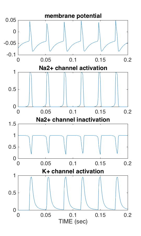
subplot(4,1,1)
plot(t, state(:,1)); axis([0 t(end) -.1 .05]);
title('membrane potential')
subplot(4,1,2)
plot(t, state(:,2)); axis([0 t(end) -.1 1.1]);
title('Na2+ channel activation')
subplot(4,1,3)
plot(t, state(:,3)); axis([0 t(end) -.1 1.1]);
title('Na2+ channel inactivation')
subplot(4,1,4)
plot(t, state(:,4)); axis([0 t(end) -.1 1.1]);
title('K+ channel activation')
xlabel('TIME (sec)')