Local Minima

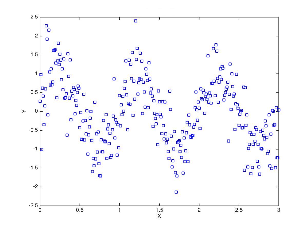
Generate (x,y) data by adapting the following MATLAB code to your language of choice:

x = 0:0.01:3;
y = sin(2*pi*x) + randn(size(x))*0.5;

Here’s what the data look like (yours may look slightly different since the y values involve random values):

Your task is to fit a function of the following form to the data:

\[ \hat{y} = \mathrm{sin}(\beta x) \]

The (single) parameter to be optimized is \(\beta\). Your cost function \(J\) is:

\[ J = \sum_{i=1}^{n} (\hat{y_{i}} - y_{i})^{2} \]

where \(n\) is the number of \((x,y)\) pairs in the data.

Map the cost landscape

Compute the cost function \(J\) for values of \(\beta\) ranging from -10.0 to 10.0 in steps of 0.01, and plot the cost landscape (plot \(J\) as a function of \(\beta\)).

Optimize for beta

Use whatever optimization approach/method you wish, to find the value of \(\beta\) that minimizes the cost function \(J\).

Plot the fit

Plot the data (\(x\) vs \(y\)) and overlay a plot of the best fitting function (\(x\) vs \(\hat{y}\)). Provide a rationale for why you think that you have found the global minimum and not a local minimum.