
Fall, 2021
Systems can be characterized by the specific relation between their input(s) and output(s). A static system has an output that only depends on its input. A mechanical example of such a system is an idealized, massless spring. The length of the spring depends only on the force (the input) that acts upon it. Change the input force, and the length of the spring will change, and this will happen instantaneously (obviously a massless spring is a theoretical construct). A system becomes dynamical (it is said to have dynamics) when a mass is attached to the spring (Figure 1 below). Now the position of the mass (and equivalently, the length of the spring) is no longer directly dependent on the input force, but is also tied to the acceleration of the mass, which in turn depends on the sum of all forces acting upon it (the sum of the input force and the force due to the spring). The net force depends on the position of the mass, which depends on the length of the spring, which depends on the spring force. The property that acceleration of the mass depends on its position makes this a dynamical system.
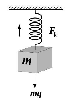
Dynamical systems can be characterized by differential equations that relate the state derivatives (e.g. velocity or acceleration) to the state variables (e.g. position). The differential equation for the spring-mass system depicted above is:
\[m\ddot{x} = -kx + mg\]
Where \(x\) is the position of the mass \(m\) (the length of the spring), \(\ddot{x}\) is the second derivative of position (i.e. acceleration), \(k\) is a constant (related to the stiffness of the spring), and \(g\) is the graviational constant (9.81 m/s/s).
The system is said to be a second order system, as the highest derivative that appears in the differential equation describing the system, is two. The position \(x\) and its time derivative \(\dot{x}\) are called states of the system, and \(\dot{x}\) and \(\ddot{x}\) are called state derivatives.
Most systems out there in nature are dynamical systems. For example most chemical reactions under natural circumstances are dynamical: the rate of change of a chemical reaction depends on the amount of chemical present, in other words the state derivative is proportional to the state. Dynamical systems exist in biology as well. For example the rate of change of the population size of a certain species likely depends on its population size.
Dynamical equations are often described by a set of coupled differential equations. For example, the reproduction rate of rabbits (state derivative 1) depends on the population of rabbits (state 1, \(x\)) and on the population size of foxes (state 2, \(y\)). The reproduction rate of foxes (state derivative 2, \(\dot{y}\)) depends on the population of foxes (state 2, \(y\)) and also on the population of rabbits (state 1, \(x\)). In this case we have two coupled first-order differential equations, and hence a system of order two. The so-called predator-prey model is also known as the Lotka-Volterra equations:
\[\begin{aligned} \dot{x} &= x(\alpha - \beta y)\\ \label{eq:lotkavolterra1} \dot{y} &= -y(\gamma - \delta x) \end{aligned}\]
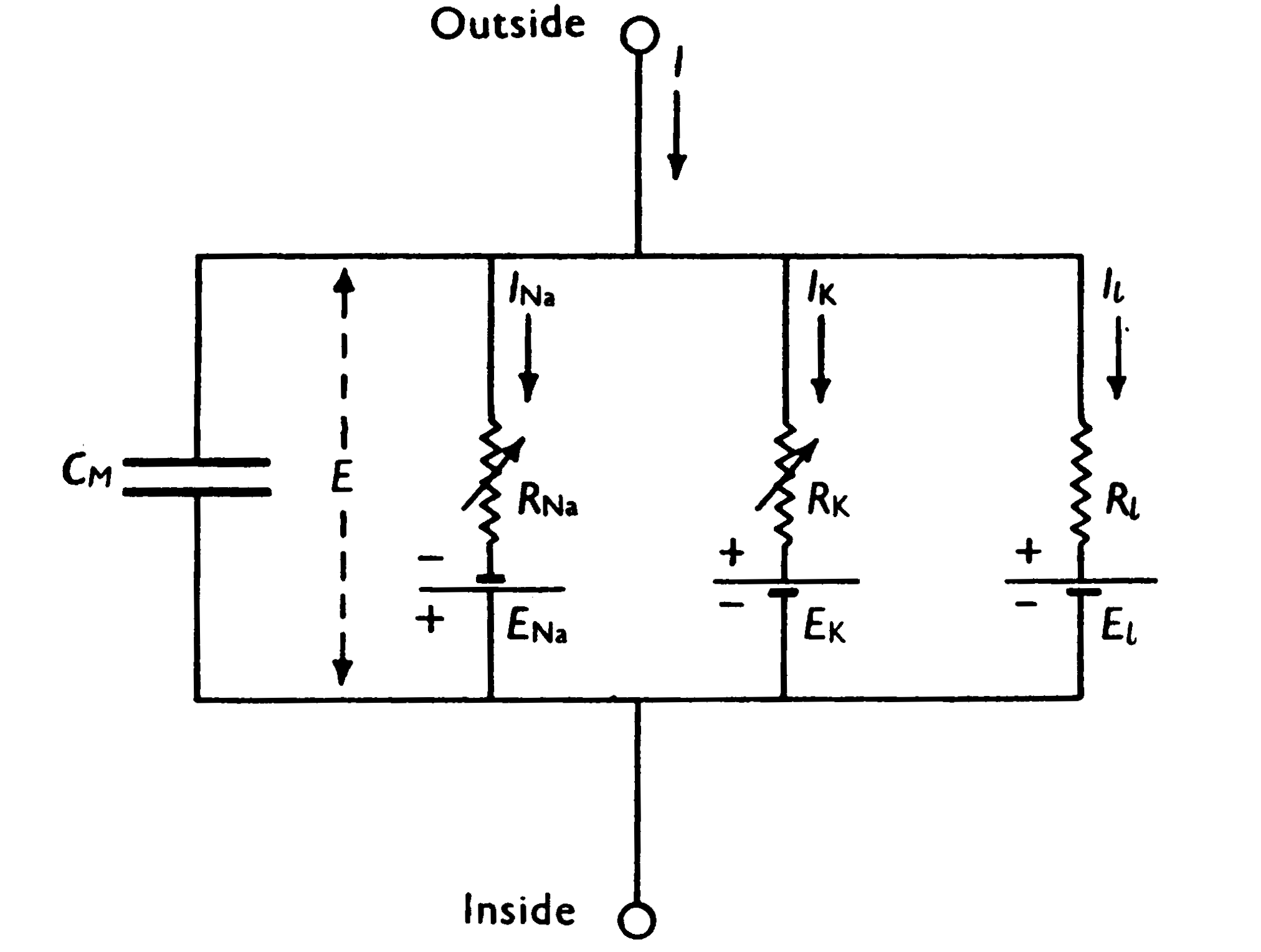
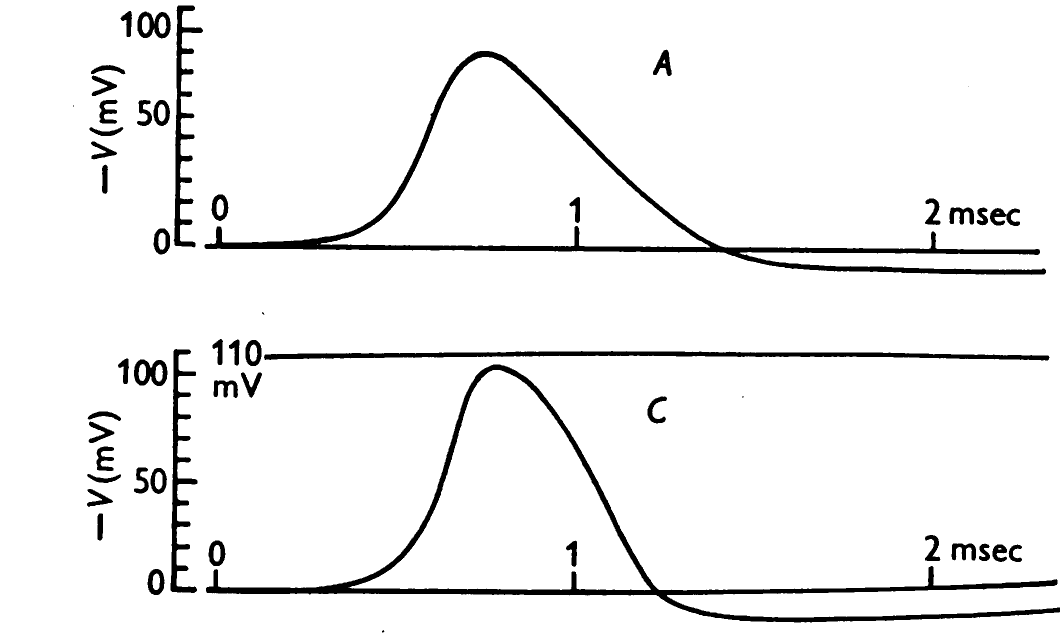
There are two main reasons why we would want to model a physical system using mathematical equations, one being practical and one mostly theoretical. The practical use is prediction. A typical example of a dynamical system that is modelled for prediction is the weather. The weather is a very complex, (high-order, nonlinear, coupled and chaotic) system. More theoretically, one reason to make models is to test the validity of a functional hypothesis of an observed phenomenon. A beautiful example is the model made by Hodgkin and Huxley to understand how action potentials arise and propagate in neurons (see Figures 2 and 3 below). They modelled the different (voltage-gated) ion channels in an axon membrane and showed using mathematical models that indeed the changes in ion concentrations were responsible for the electrical spikes observed experimentally 7 years earlier.
A second theoretical reason to make models is that it is sometimes very difficult, if not impossible, to answer a certain question empirically. As an example we take the following biomechanical question: Would you be able to jump higher if your biceps femoris (part of your hamstrings) were two separate muscles each crossing only one joint rather than being one muscle crossing both the hip and knee joint? Not a strange question as one could then independently control the torques around each joint.
In order to answer this question empirically, one would like to do the following experiment:
measure the maximal jump height of a subject
change only the musculoskeletal properties in question
measure the jump height again
Of course, such an experiment would yield several major ethical, practical and theoretical drawbacks. It is unlikely that an ethics committee would approve the transplantation of the origin and insertion of the hamstrings in order to examine its effect on jump height. And even so, one would have some difficulties finding subjects. Even with a volunteer for such a surgery it would not bring us any closer to an answer. After such a surgery, the subject would not be able to jump right away, but would have to undergo significant rehabilitation, and surely during such a period many factors will undesirably change like maximal contractile forces. And even if the subject would fully recover (apart from the hamstrings transplantation), his or her nervous system would have to find the new optimal muscle stimulation pattern.
If one person jumps lower than another person, is that because she cannot jump as high with her particular muscles, or was it just that her CNS was not able to find the optimal muscle activation pattern? Ultimately, one wants to know through what mechanism the subject’s jump performance changes. To investigate this, one would need to know, for example, the forces produced by the hamstrings as a function of time, something that is impossible to obtain experimentally. Of course, this example is somewhat ridiculous, but its message is hopefully clear that for several questions a strict empirical approach is not suitable. An alternative is provided by mathematical modelling.
Here we will be examining three systems—a mass-spring system, a two-link double pendulum system, and a system representing weather patterns. In each case we will see how to go from differential equations characterizing the dynamics of the system, to MATLAB code, and run that code to simulate the behaviour of the system over time. We will see the great power of simulation, namely the ability to change aspects of the system at will, and simulate to explore the resulting change in system behaviour.
A dynamical system such as the mass-spring system we saw before, can be characterized by the relationship between state variables \(s\) and their (time) derivatives \(\dot{s}\). How do we arrive at the correct characterization of this relationship? The short answer is, we figure it out using our knowledge of physics, or we are simply given the equations by someone else. Let’s look at a simple mass-spring system again, shown in Figure 4.
We know a couple of things about this system. We know from Hooke’s law of elasticity that the extension of a spring is directly and linearly proportional to the load applied to it. More precisely, the force that a spring applies in response to a perturbation from it’s resting length (the length at which it doesn’t generate any force), is linearly proportional, through a constant \(k\), to the difference in length between its current length and its resting length (let’s call this distance \(x\)). For convention let’s assume positive values of \(x\) correspond to lengthening the spring beyond its resting length, and negative values of \(x\) correspond to shortening the spring from its resting length.
\[F = -kx\]
Let’s decide that the state variable that we are interested in for our system is \(x\).
We also know from Newton’s laws of motion (specifically Newton’s second law) that the net force on an object is equal to its mass \(m\) multiplied by its acceleration \(a\) (the second derivative of position).
\[F = ma\]
Instead of using \(a\) to denote acceleration let’s use a different notation, in terms of the spring’s perturbed length \(x\). The rate of change (velocity) is denoted \(\dot{x}\) and the rate of change of the velocity (i.e. the acceleration) is denoted \(\ddot{x}\).
\[F = m \ddot{x}\]
We also know that the mass is affected by two forces: the force due to the spring (\(-kx\)) and also the gravitational force \(g\). So the equation characterizing the net forces on the mass is
\[\sum{F} = m\ddot{x} = -kx + mg\]
or just
\[m\ddot{x} = -kx + mg\]
This equation is a second-order differential equation, because the highest state derivative is a second derivative (i.e. \(\ddot{x}\), the second derivative, i.e. the acceleration, of \(x\)). The equation specifies the relationship between the state variables (in this case a single state variable \(x\)) and its derivatives (in this case a single derivative, \(\ddot{x}\)).
The reason we want an equation like this, from a practical point of view, is that we will be using numerical solvers in MATLAB to integrate this differential equation over time, so that we can simulate the behaviour of the system. What these solvers need is a MATLAB function that returns state derivatives, given current states. We can re-arrange the equation above so that it specifies how to compute the state derivative \(\ddot{x}\) given the current state \(\ddot{x}\).
\[\ddot{x} = \frac{-kx}{m} + g\]
Now we have what we need in order to simulate this system in MATLAB. At any time point, we can compute the acceleration of the mass by the formula above.
Here is a MATLAB function that we will be using to simulate the mass-spring system. All it does, really, is compute the equation above: what is the value of \(\ddot{x}\), given \(x\)? The one addition we have is that we are going to keep track not just of one state variable \(x\) but also its first derivative \(\dot{x}\) (the rate of change of \(x\), i.e. velocity).
function stated = MassSpring(t, state)

  % unpack the state vector
  x  = state(1); % position
  xd = state(2); % velocity

  % these are our constants
  k = 2.5; % Newtons per metre
  m = 1.5; % Kilograms
  g = 9.8; % metres per second per second

  % compute acceleration xdd
  xdd = ((-k*x)/m) + g;

  stated = [xd; xdd]; % velocity; acceleration

end
Note that the function we wrote takes two arguments as inputs: state and t, which corresponds to time. This is necessary for the numerical solver that we will use in MATLAB. The state variable is actually an array of two values corresponding to \(x\) and \(\dot{x}\).
How does numerical integration (simulation) work?
The simplest method is called the Euler method named after Leonhard Euler, the 18th century Swiss mathematician. In the Euler method, the state estimate for the next time period \(x_{n+1}\) is equal to the state from the previous time period \(x_{n}\) plus the product of the state derivative \(\dot{x_{n}}\) and the change-in-time (step size) \(\Delta{t}\):
\[ x_{n+1} = x_{n} + \Delta{t}(\dot{x_{n}}) \]
In this way, numerical solvers esimate how the system states \((x,\dot{x})\) unfold over time, given the initial conditions, and the known relationship between state derivatives and system states.
The Euler method is an approximation, and its accuracy increases as the step size decreases. It turns out that for many dynamical systems, other methods are far more accurate, and more stable, for example the Runge-Kutta family of methods.
Runge-Kutta and other integration algorithms are readily available in MATLAB and are known as ODE solvers (ODE stands for ordinary differential equation).
Here’s how we would simulate the mass-spring system above, using the Runge-Kutta method. Assume that we have the function MassSpring.m defined as above:
state0 = [0.0, 0.0];
t = 0:.1:10;

[t,state] = ode45('MassSpring', t, state0);

plot(t, state)
xlabel('TIME (sec)')
ylabel('STATES')
title('Mass-Spring System')
legend({'$x$ (m)', '$\dot{x}$ (m/sec)'},'interpreter','latex')
A couple of notes about the code. I have simply chosen, out of the blue, values for the constants \(k\) and \(m\). The gravitational constant \(g\) is of course known. I have also chosen to simulate the system for 10 seconds, and I have chosen a time resolution of 100 milliseconds (0.1 seconds). We will talk later about the issue of what is an appropriate time resolution for simulation.
You should see a plot like the one shown in Figure 5 below.
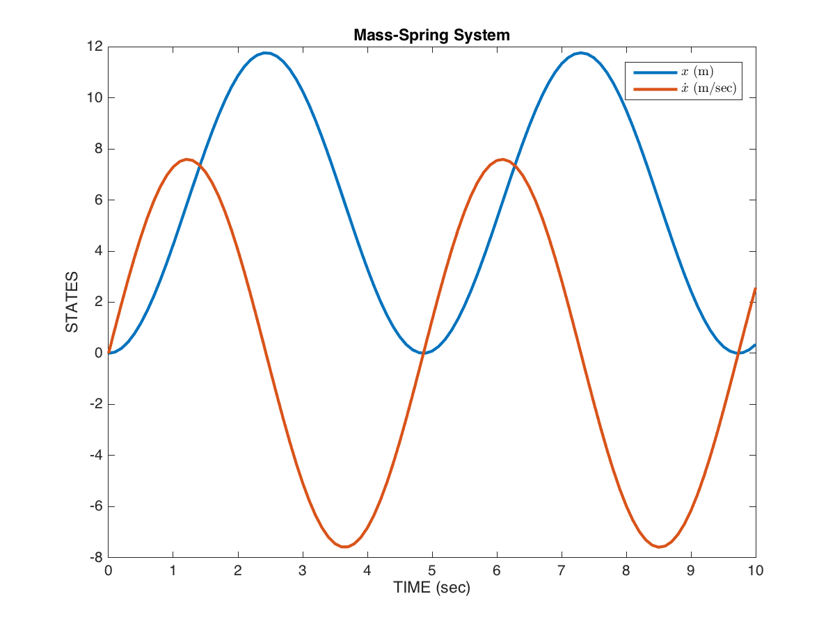
The blue line shows the position \(x\) of the mass (the length of the spring) over time, and the orange line shows the rate of change of \(x\), in other words the velocity \(\dot{x}\), over time. These are the two states of the system, simulated over time.
The way to interpret this simulation is, if we start the system at \(x=0\) and \(\dot{x}=0\), and simulate for 10 seconds, this is how the system would behave.
Now you can appreciate the power of mathematical models and simulation: given a model that characterizes (to some degree of accuracy) the behaviour of a system we are interested in, we can use simulation to perform experiments in simulation instead of in reality. This can be very powerful. We can ask questions of the model, in simulation, that may be too difficult, or expensive, or time consuming, or just plain impossible, to do in real-life empirical studies. The degree to which we regard the results of simulations as interpretable, is a direct reflection of the degree to which we believe that our mathematical model is a reasonable characterization of the behaviour of the real system.
Here is a MATLAB function called double_pendulum.m that implements the forward dynamics of a double pendulum. You can look up the equations of motion on the Wikipedia page. The code below simply implements these equations. It’s not important right now to understand where the equations came from, but know that they can be derived from a relatively basic knowledge of physics. One property of a double pendulum is that the motion about one joint affects the motion of the adjacent joint, and vice-versa. These interaction forces can result in complex behaviour. Indeed, experimental work has demonstrated that the nervous system is capable of predicting these interaction forces and compensating for them (or in some cases exploiting them) during voluntary movements of the upper limb.
The four state variables are the angle of joint 1, the angle of joint 2, the velocity of joint 1 and the velocity of joint 2.
function stated = double_pendulum(t, state)

a1 = state(1);
a2 = state(2);
a1d = state(3);
a2d = state(4);

damping = 0.0;
g = 9.8;

% inertia matrix
M = [3 + 2*cos(a2), 1+cos(a2); ...
     1+cos(a2), 1];

% coriolis, centripetal and gravitational forces
c1 = a2d*((2*a1d) + a2d)*sin(a2) + ...
     2*g*sin(a1) + g*sin(a1+a2);
c2 = -(a1d^2)*sin(a2) + g*sin(a1+a2);

% passive dynamics
cc = [c1-damping*a1d; ...
      c2-damping*a2d];

% compute accelerations
acc = M\cc;

stated = [a1d; a2d; acc(1); acc(2)];

end
Now that we have a function that implements the equations of motion, now we can run a simulation, by starting the arm out at some initial condition (initial joint angles and initial joint velocities) and integrating the differential equations over time (using MATLAB’s ode45 function). Here is some MATLAB code for running a simulation from a given set of initial state conditions, and animating the result in a figure window. You’ll need this helper function called a2h.m as well:
function [h0,h1,h2] = a2h(a1,a2)

h0 = [0,0];
h1 = [sin(a1), cos(a1)];
h2 = [sin(a1) + sin(a1+a2), ...
      cos(a1) + cos(a1+a2)];

end
Here is the script for running the simulation and generating the animation:
%% run a simulation of a double pendulum

t = 0:.01:10;
x0 = [pi, pi/2, 0, 0];
[t,x] = ode45('double_pendulum', t, x0);

%% plot states over time

figure
plot(t,x)

%% run an animation

figure('position',[62 855 965 333]);
subplot(1,2,1)
plot(t,x(:,1:2))
legend({'a1','a2'})
hold on
s1ylim = get(gca,'ylim');
tline = plot([0 0],s1ylim,'r-','linewidth',1);
subplot(1,2,2)
[h0,h1,h2] = a2h(x(1,1),x(1,2));
l1 = plot([h0(1) h1(1)],[h0(2) h1(2)],'b-');
hold on
l2 = plot([h1(1) h2(1)],[h1(2) h2(2)],'b-');
axis([-2.2 2.2 -2.2 2.2]); axis equal
p0 = plot(h0(1),h0(2),'k.','markersize',15);
p1 = plot(h1(1),h1(2),'b.','markersize',15);
p2 = plot(h2(1),h2(2),'r.','markersize',15);
tp = title(sprintf('%5.1f',t(1)));
skip = 3;
for i=1:skip:length(t)
    subplot(1,2,1)
    set(tline, 'Xdata', [t(i) t(i)]);
    set(tline, 'Ydata', s1ylim);
    subplot(1,2,2)
    [h0,h1,h2] = a2h(x(i,1), x(i,2));
    set(l1, 'XData', [h0(1) h1(1)]);
    set(l1, 'YData', [h0(2) h1(2)]);
    set(l2, 'XData', [h1(1) h2(1)]);
    set(l2, 'YData', [h1(2) h2(2)]);
    set(p1, 'XData', h1(1));
    set(p1, 'YData', h1(2));
    set(p2, 'XData', h2(1));
    set(p2, 'YData', h2(2));
    set(tp, 'String', sprintf('%5.1f', t(i)));
    axis([-2.2 2.2 -2.2 2.2]);
    drawnow;
end
What you see is a window with the time-varying angles on the left panel and an animation of the double pendulum on the right panel, as in Figure 6.
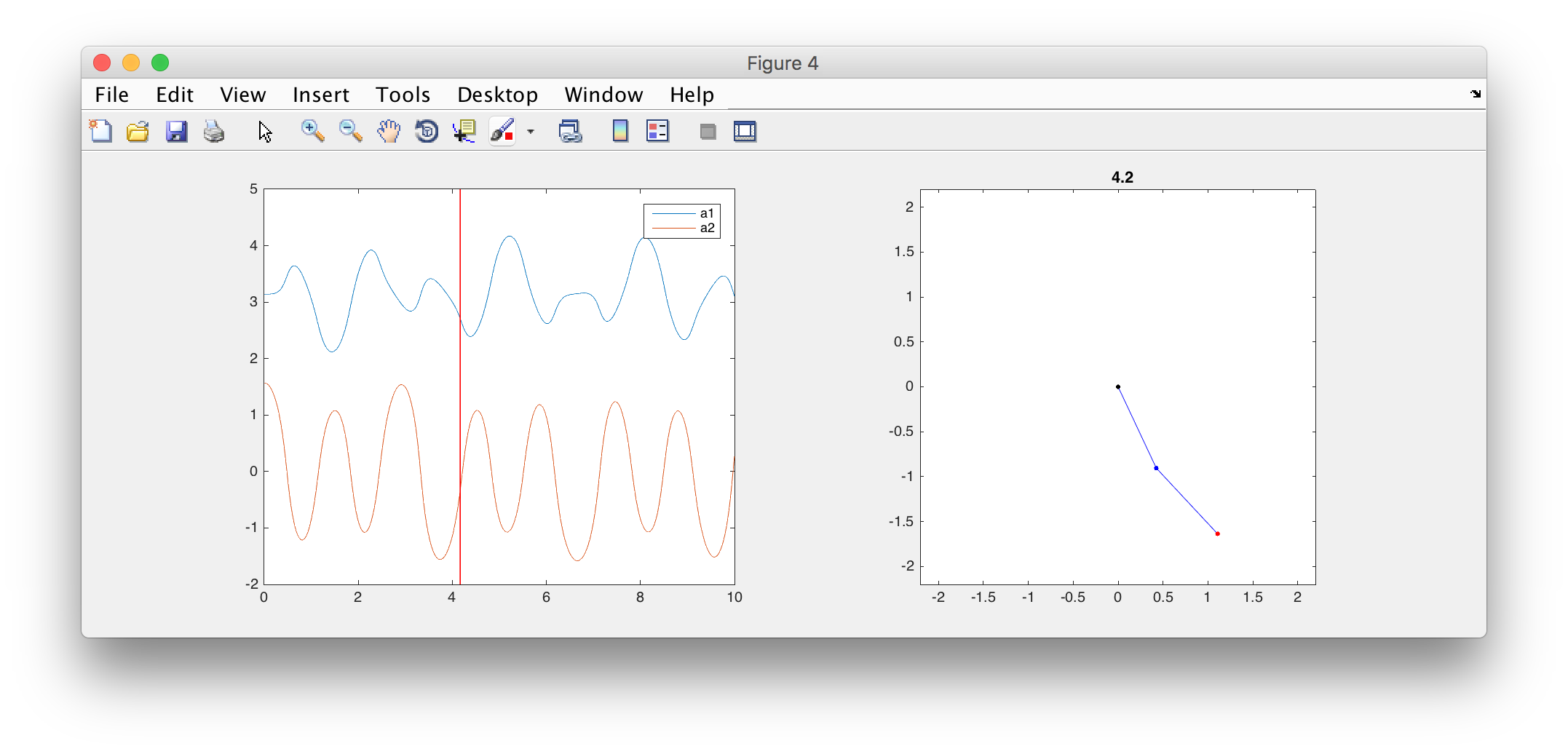
Play with the simulation code and see what happens when you start the simulation from different initial conditions, for example different initial joint angles.
The simple model described here has only passive motion, there are no active forces (for example generated by muscles). One can relatively easily add mathematical models of muscle force generation, and other neurophysiologically relevant properties such as muscle mechanics, spinal reflex circuitry, reflex time delays, and so on. One can then use such a model to test hypotheses about how the brain controls voluntary arm movement.
The Lorenz system is a dynamical system that we will look at briefly, as it will allow us to discuss several interesting issues around dynamical systems. It is a system often used to illustrate non-linear systems theory and chaos theory. It’s sometimes used as a simple demonstration of the butterfly effect (sensitivity to initial conditions). See here for a YouTube video that explains the meaning of the \(x\), \(y\) and \(z\) coordinates.
The Lorenz system is a simplified mathematical model for atmospheric convection. Let’s not worry about the details of what it represents, for now the important things to note are that it is a system of three coupled differential equations, and characterizes a system with three state variables \((x,y,z\)).
\[\begin{aligned} \dot{x} &= &\sigma(y-x)\\ \dot{y} &= &(\rho-z)x - y\\ \dot{z} &= &xy-\beta z\end{aligned}\]
If you set the three constants \((\sigma,\rho,\beta)\) to specific values, the system exhibits chaotic behaviour.
\[\begin{aligned} \sigma &= &10\\ \rho &= &28\\ \beta &= &\frac{8}{3}\end{aligned}\]
Let’s implement this system in MATLAB. We have been given above the three equations that characterize how the state derivatives \((\dot{x},\dot{y},\dot{z})\) depend on \((x,y,z)\) and the constants \((\sigma,\rho,\beta)\). All we have to do is write a function that implements this, set some initial conditions, decide on a time array to simulate over, and run the simulation using ode45(). First the function myLorenz.m that defines the differential equations:
function stated = myLorenz(t, state)
 x = state(1);
 y = state(2);
 z = state(3);

 % these are our constants
 sigma = 10.0;
 rho = 28.0;
 beta = 8/3;

 % compute the state derivatives
 xd = sigma * (y-x);
 yd = (rho-z)*x - y;
 zd = x*y - beta*z;

 % return the state derivatives
 stated = [xd; yd; zd];
end
Now the code to run the simulation:
state0 = [2.0, 3.0, 4.0];
t = 0:.01:30;

[t,state] = ode45('myLorenz', t, state0);

% plot the resuling state-space trajectory in 3D
plot3(state(:,1), state(:,2), state(:,3))
xlabel('X'); ylabel('Y'); zlabel('Z');
grid on
You should see something like the plot shown in Figure 7 below.
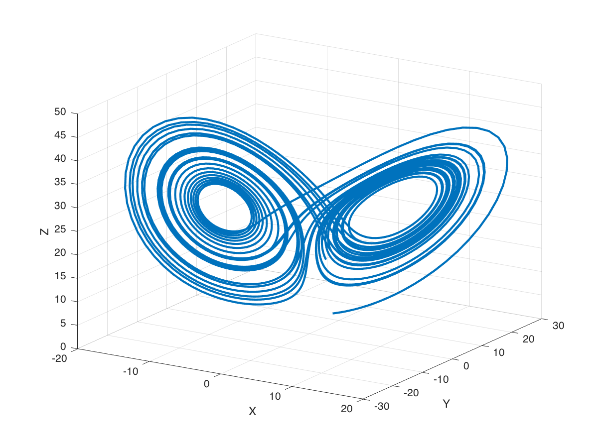
The three axes on the plot represent the three states \((x,y,z)\) plotted over the 30 seconds of simulated time. We started the system with three particular values of \((x,y,z)\) (I chose them arbitrarily), and we set the simulation in motion. This is the trajectory, in state-space, of the Lorenz system.
You can see an interesting thing … the system seems to have two stable equilibrium states, or attractors: those circular paths. The system circles around in one “neighborhood” in state-space, and then flips over and circles around the second neighborhood. The number of times it circles in a given neighborhood, and the time at which it switches, displays chaotic behaviour, in the sense that they are exquisitly sensitive to initial conditions.
For example let’s re-run the simulation but change the initial conditions. Let’s change them by a very small amount, say 0.0001 … and let’s only change the \(x\) initial state by that very small amount. We will simulate again for 30 seconds.
state0 = [2.0, 3.0, 4.0];
t = 0:.01:30;

[t,state] = ode45('myLorenz', t, state0);

% plot the resuling state-space trajectory in 3D
plot3(state(:,1), state(:,2), state(:,3), 'b-', 'linewidth', 2)
xlabel('X'); ylabel('Y'); zlabel('Z');
grid on

% re-run with very small change in initial conditions
delta = 0.0001;

state0 = [2.0+delta, 3.0, 4.0];
t = 0:.01:30;

[t2,state2] = ode45('myLorenz', t, state0);

hold on
plot3(state2(:,1), state2(:,2), state2(:,3), 'r-', 'linewidth', 2)
You should see something like what is shown in Figure 8 below.
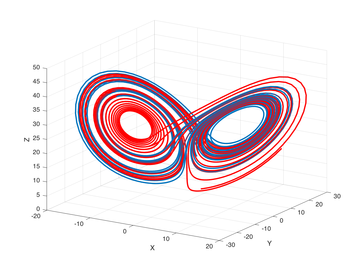
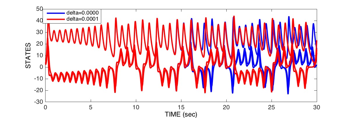
You can sort of see that at some point the two state-space trajectories diverge. You can better visualize this by plotting each state against time as shown in Figure 9.
But let’s go one step further, let’s plot the distance between each point in state-space as a function of time:
dist = sqrt(sum((state2-state).^2,2));
figure
plot(t,dist,'b-','linewidth',2)
xlabel('TIME (sec)')
ylabel('DISTANCE')
grid on
You’ll see something like what’s shown in Figure 10.
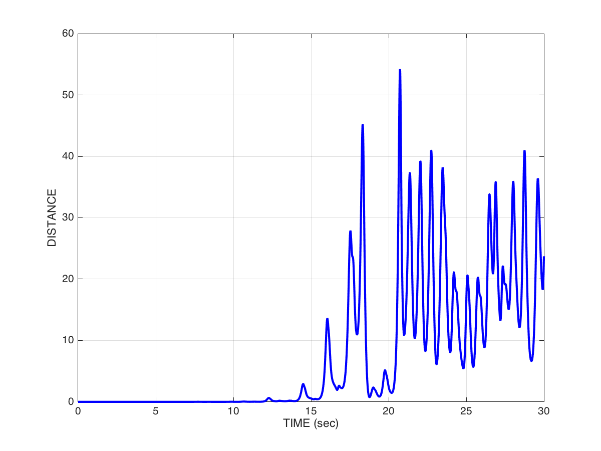
If you look at the peaks, we see that up until the 15 second mark or so, the two trajectories are basically aligned, and then afterwards, they suddenly diverge, and quite significantly. We have distances in the range of 30, 40 or even 50 units—and remember, this is generated with a difference in initial conditions of only 0.0001. That’s a 500,000x change.
Here’s some MATLAB code to generate an animation:
figure
plot3(state(:,1),state(:,2),state(:,3),'b-');
hold on
plot3(state2(:,1),state2(:,2),state2(:,3),'r-');
p1 = plot3(state(1,1),state(1,2),state(1,3),'b.','markersize',30);
p2 = plot3(state2(1,1),state2(1,2),state2(1,3),'r.','markersize',30);
tt = title('0.0');
step = 1;
view([32 22])
grid on
xlabel('X'); ylabel('Y'); zlabel('Z');
drawnow
for i=1:step:length(t)
    set(p1,'XData',state(i,1));
    set(p1,'YData',state(i,2));
    set(p1,'ZData',state(i,3));
    set(p2,'XData',state2(i,1));
    set(p2,'YData',state2(i,2));
    set(p2,'ZData',state2(i,3));
    set(tt,'String',sprintf('%6.2f',t(i)));
    drawnow
end
You should see an animation of the two state-space trajectories.
The original simulation is shown in blue. The simulation with the altered initial condition is in red. Then an animated filled circle shows the state space over time for the original (blue) and new (red, in which the initial condition of \(x\) was increased by 0.0001). The two follow each other quite closely for a long time, and then begin to diverge at about the 16 second mark. At the 20.76 second mark they look like what’s shown in Figure 11.
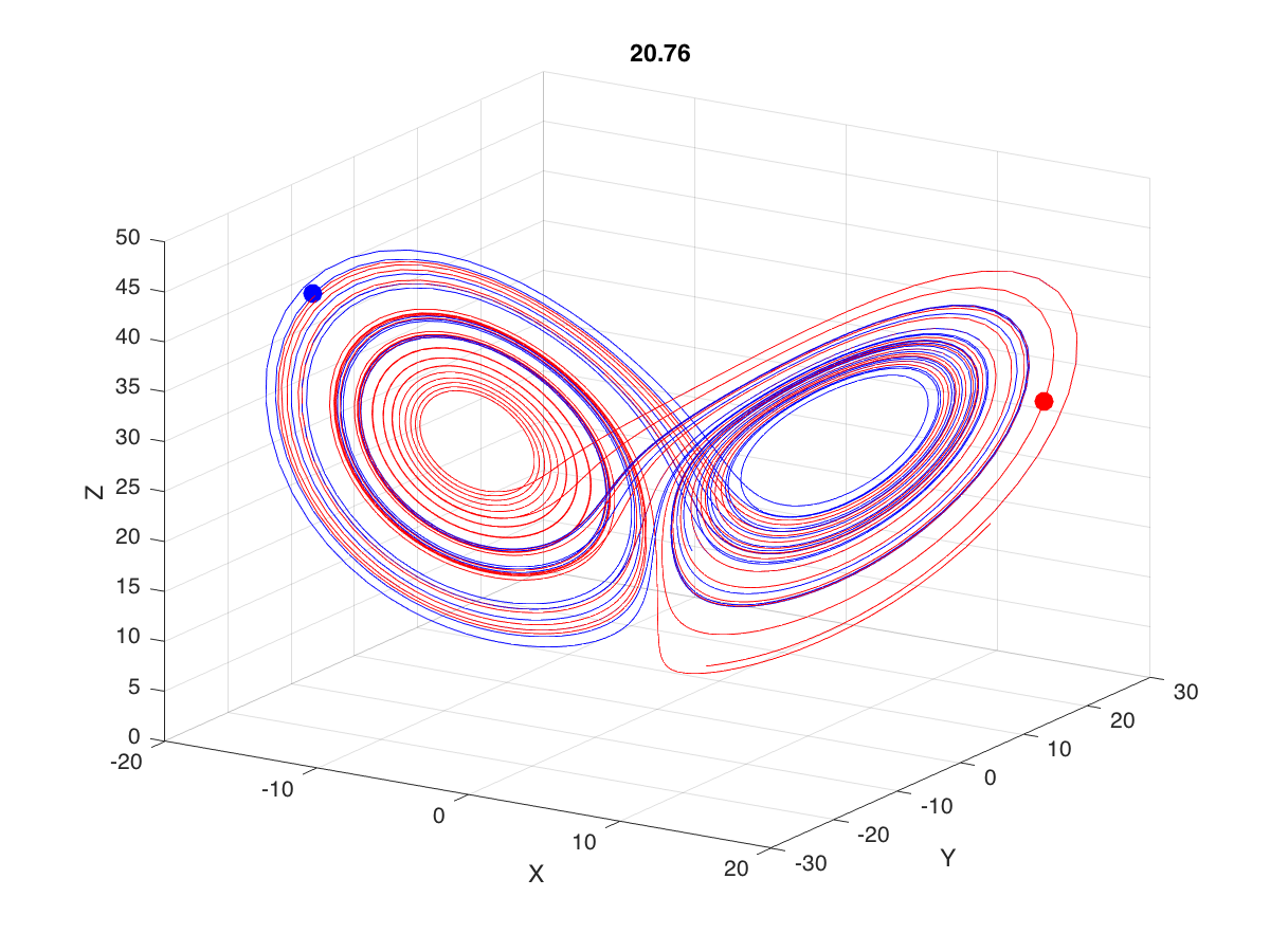
Note how the two systems are in different neighborhoods entirely!
This has illustrated how systems with relatively simple differential equations characterizing their behaviour, can turn out to be exquisitely sensitive to initial conditions. Just imagine if the initial conditions of your simulation were gathered from empirical observations (like the weather, for example). Now imagine you use a model simulation to predict whether it will be sunny (left-hand neighborhood of the plot above) or thunderstorms (right-hand neighborhood), 30 days from now. If the answer can flip between one prediction and the other, based on a 1/10,000 different in measurement, you had better be sure of your empirical measurement instruments, when you make a prediction 30 days out! Actually this won’t even solve the problem, no matter how precise your measurements. The point is that the system as a whole is very sensitive to even tiny changes in initial conditions. This is one reason why short-term weather forecasts are relatively accurate, but forecasts past a couple of days can turn out to be dead wrong.
thanks to Dinant Kistemaker for co-authoring this topic