
Fall, 2021
In this chapter we will look at ways of solving problems with your code using the various debugging tools in MATLAB. We will also look at profiling your code using the built-in profiler in MATLAB, which can be used to identify parts of your code that are taking the most time to execute. We will go over a number of ways to make sure your code runs fast. In some cases this amounts to telling you about what not to do to make your code run slow. Finally we will look at the MATLAB Coder, which is a toolbox included in MATLAB that can generate standalone C and C++ code from MATLAB code. It can also generate so-called binary MEX functions that allow you to call compiled versions of your MATLAB code, potentially speeding up computations.
There are at least two kinds of errors you will encounter in programming. The first is when you run your code and it aborts because of some kind of error, and you recieve an error message. Sometimes those error messages are useful and you can determine immediately what is wrong. Other times the error message is cryptic and it takes some detective work on your part to figure out what part of the code is failing, and why it is failing.
The second type of error is when your code runs without aborting, and without reporting any problem to you, but you do not get the expected result. This is much more difficult to debug.
In general the approach you should use for debugging is to step through your code, line by line, and ensure that each step is (a) performing the operation you think it is, and (b) is performing the appropriate operation.
The built-in MATLAB editor that you can use to edit your MATLAB code files has a handy feature called breakpoints that allows you to set a breakpoint (or multiple breakpoints) on a specific line (or lines) of your code, such that as you run your code, MATLAB stops at a breakpoint and enters a special mode called the debugger. Once in the debugger you can examine values of variables, step to the next line of code, step in or out of functions, and continue executing the rest of the code. It’s a very useful way to halt execution at specific places in your code, so that you can examine what is going on. Often this is how will find bugs and errors in your code—when you assumed a variable had a specific value, or an operation resulted in a specific value, and in fact it didn’t.
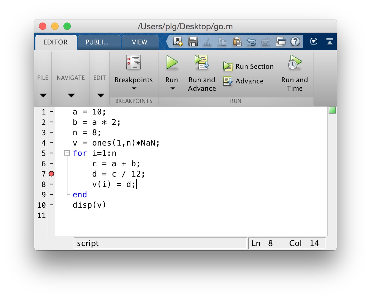
Here is an example of a MATLAB script called go.m which computes some values, and executes a for–loop in which is fills a vector v with some numbers. By clicking with the mouse on the little dash (-) next to the line number 7 (on the left hand side of the editor window) I have inserted a breakpoint, which appears as a filled red circle.
Now when we run the program, MATLAB stops the first time it encounters the breakpoint on line 7. You will see this at the MATLAB command prompt:
>> go
7       d = c / 12;
K>>
It reports the line number (7) and the code appearing on that line, and it puts you in to debugger mode, as indicated by the prompt K>>. Now you can enter the names of variables to query their value, for example we can see what the value of i, and c are:
K>> i

i =

     1

K>> c

c =

    30
We can step to the next line of code by clicking on the “Step” button appearing at the top of the editor window, as shown here:
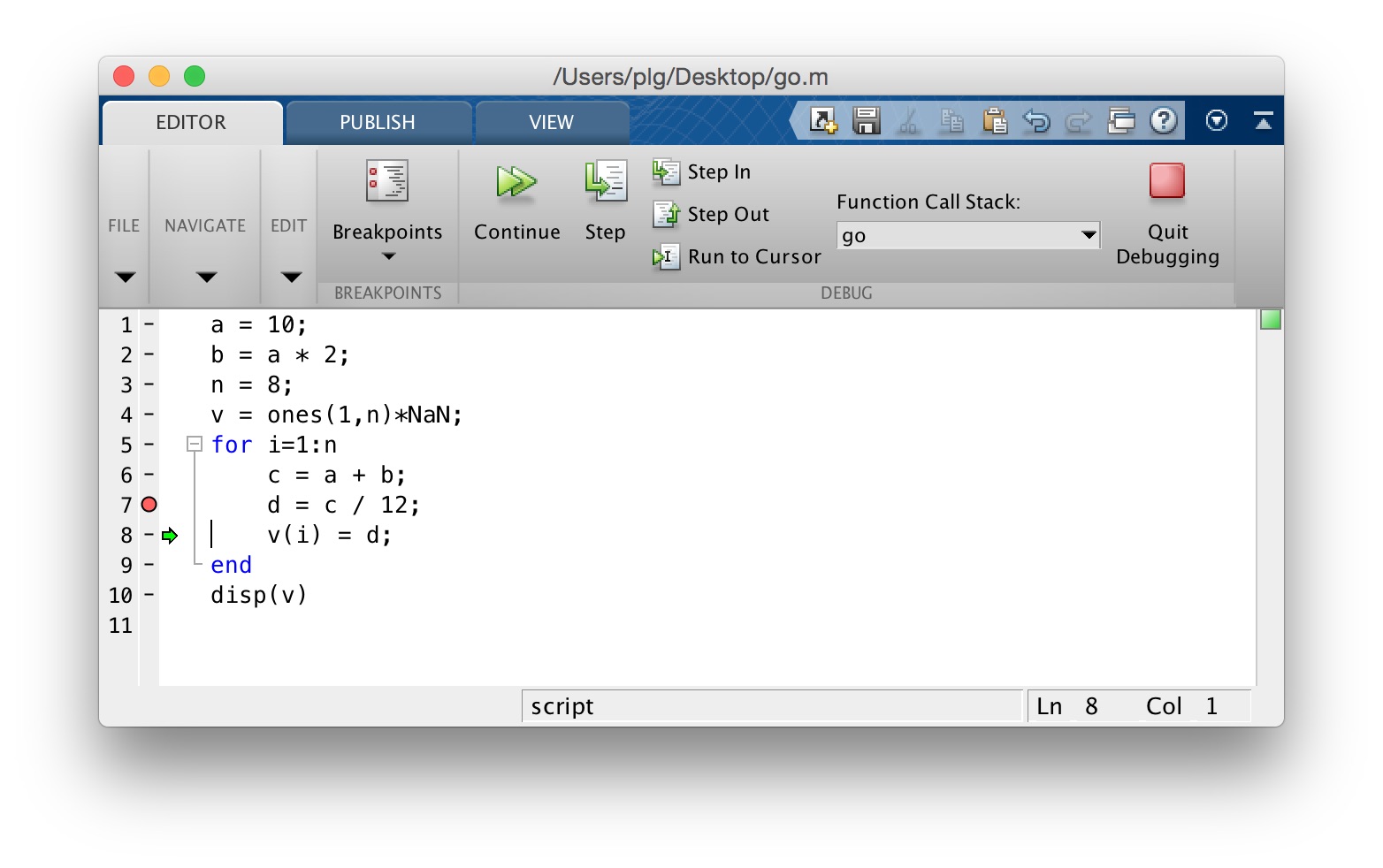
You will see that there is now a little green arrow pointing to the right, at line 8 in the code. This indicates the line of code where the debugger has stopped, and is waiting for you to tell it what to do next. We can click on the “Continue” button at the top of the editor window to continue. When we do this we see that MATLAB has stopped again, at line 7 again, as shown here:

At the command prompt we can enter i to query the value of i and we see that indeed we are now at iteration 2 of the for–loop:
K>> i
i =
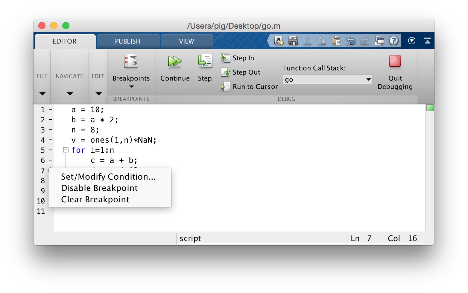
2If we click “Continue” again we will stop again at line 7, at the third iteration of the for–loop, and so on. To continue without stopping at the breakpoint each time, we need to remove or disable the breakpoint. Right-click on the little red circle and a pop-up menu gives you these options. Note that there is also an option called “Set/Modify Condition...”—this allows you to specify a logical condition which if true, will cause MATLAB to stop at the breakpoint, otherwise not. This is a nice way to set up breakpoints that only stop the code if certain conditions are met—for example if the value of a variable you know should never be negative, is less than zero.
The MathWorks online documentation has a page devoted to debugging here:
One obvious way of speeding up your MATLAB programs is to first identify the pieces of your program that are slowest—and then do what you can to speed up those parts.
tic and tocOne way to time your code is to use the tic and toc commands in MATLAB.
>> help tic
 tic Start a stopwatch timer.
    tic and TOC functions work together to measure elapsed time.
    tic, by itself, saves the current time that TOC uses later to
    measure the time elapsed between the two.

    TSTART = tic saves the time to an output argument, TSTART. The
    numeric value of TSTART is only useful as an input argument
    for a subsequent call to TOC.

    Example: Measure the minimum and average time to compute a sum
             of Bessel functions.

      REPS = 1000; minTime = Inf; nsum = 10;
      tic;
      for i=1:REPS
        tstart = tic;
        sum = 0; for j=1:nsum, sum = sum + besselj(j,REPS); end
        telapsed = toc(tstart);
        minTime = min(telapsed,minTime);
      end
      averageTime = toc/REPS;

    See also toc, cputime.

    Reference page in Help browser
       doc tic
>> help toc
toc Read the stopwatch timer.
TIC and toc functions work together to measure elapsed time.
toc, by itself, displays the elapsed time, in seconds, since
the most recent execution of the TIC command.
T = toc; saves the elapsed time in T as a double scalar.
toc(TSTART) measures the time elapsed since the TIC command that
generated TSTART.
Example: Measure the minimum and average time to compute a sum
of Bessel functions.
REPS = 1000; minTime = Inf; nsum = 10;
tic;
for i=1:REPS
tstart = tic;
sum = 0; for j=1:nsum, sum = sum + besselj(j,REPS); end
telapsed = toc(tstart);
minTime = min(telapsed,minTime);
end
averageTime = toc/REPS;
See also tic, cputime.
Reference page in Help browser
doc tocThe typical pattern using tic and toc is to bracket a chunk of code you want to time with tic and toc. There are several examples in the section below on Speedy Code in which tic and toc are used to time MATLAB code execution time.
There is a tool in MATLAB called the Profiler that is very useful for showing which parts of your program take the most amount of time to execute. Think of the profiler as a way of automatically timing every part of your program and generating a handy report (which it does also).
The basic way to use the profiler is to first activate it by typing:
>> profile onYou can then run your MATLAB script, and once it is finished, stop the profiler by typing:
>> profile offYou can then generate a report by typing:
>> profile reportHere is an example using a script called go.m which calls two other functions, myfun1 and myfun2:
n = 1e4;
m = zeros(100,100);
for i=1:n
    m = m + myfun1(m);
    m = m + myfun2(m);
end
disp(sprintf('grand mean of m is %.6f\n', mean(m(:))/n));
function out = myfun1(in)
[r,c] = size(in);
tmp = randn(r,c);
for i=1:r
for j=1:c
tmp(i,j) = sqrt(tmp(i,j));
end
end
out = tmp;
endfunction out = myfun2(in)
[r,c] = size(in);
tmp = randn(r,c);
tmp = sqrt(tmp);
out = tmp;
endWe turn on the profiler, run the code, stop the profiler, and generate a report, which is shown here:
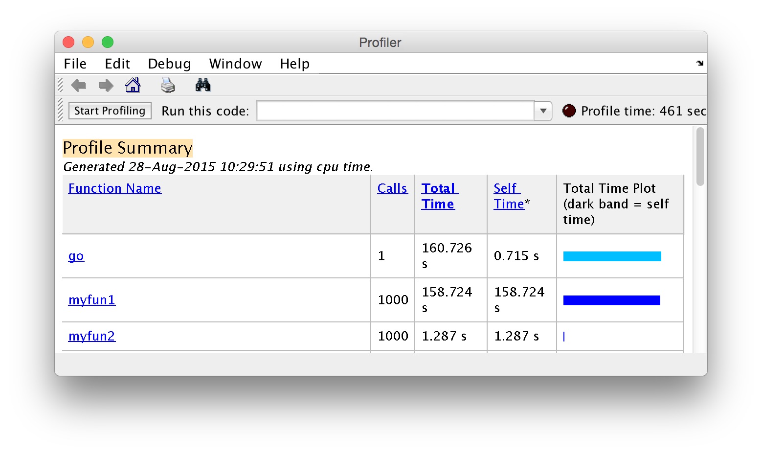
We can see that the go script overall took 160.726 seconds to run. We also see a list of functions that were called within go, and the time they took. We can see immediately that myfun1 is way slower than myfun2. If we click the mouse on myfun1 in the report, we get a new report of the myfun2 function itself, which is shown here:
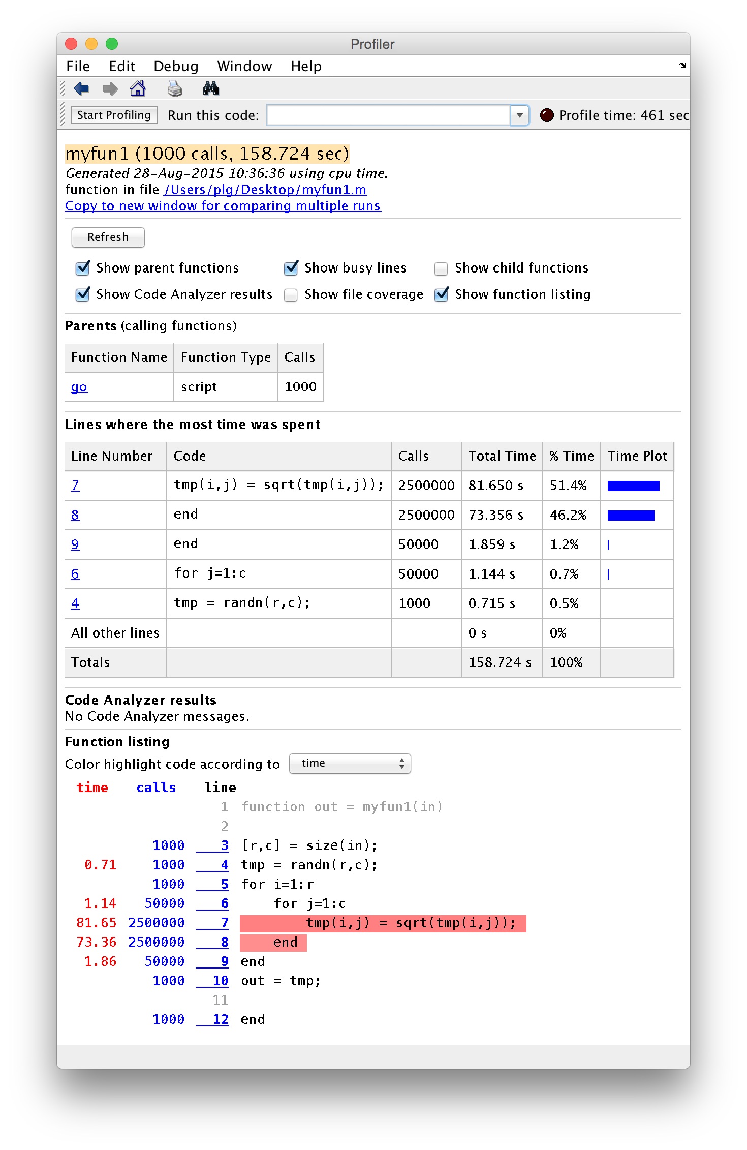
We get a quite detailed report of the lines of the code where the most time was spent. We also see the time spent, and the number of calls made to each line of code in the function.
In this case we see that line 7 of the myfun1 function is taking a lot of time to execute—this is where we take the square root of each element of a large matrix, within two nested for–loops. Line 7 represents the innermost part of these two nested for–loops, and so it’s no surprise that we are spending a lot of time here. See the section below on Vectorization for more information about how to avoid nested for–loops by using vectorized code operations.
The other way of running the profiler is by clicking with your mouse on the “Run and Time” button in the toolbar of the MATLAB code editor. The profiler will run your code, timing each line, and will open up a report window.
The MathWorks online documentation has a page on the profiler here:
Profiling for Improving Performance
There are many cases in which we want to collect the results of many computations together into a single data structure, e.g. a vector or array. One way of doing this is to start with an empty array, and each time through the loop, add a value to it (and hence lengthening it). It turns out this way is very slow. What’s much, much faster is to pre-allocate the array (and fill it with whatever values you want, e.g. 0s, or NaNs), and then set each value as you go through the loop to the result of your computation.
Here is an example in MATLAB:
% for values between 0 and n:
%
% f(i) = (i + f(i-1)) / n

n = 1e5;

% the slow way:
%
tic
c = [0];
for i=2:n
  c = [c, (i + c(i-1)) / n];
end
toc
%
% on my laptop this takes 3.605413 seconds

% the fast way, with array pre-allocation
%
tic
c = zeros(1,n);
for i=2:n
  c(i) = (i + c(i-1)) / n;
end
toc
%
% on my laptop this takes 0.002819 seconds
% this is over 1,000 times faster than the slow version
In the slow version, we start with an array of length 1 containing the number zero. Each time through the loop we concatenate the array with the next value, and in this way we build up the array.
In the fast version, we pre-allocate an array of the required length, fill it with 0s, and then each time through the loop we simply assign the appropriate value to the appropriate array position.
The reason the slow version is so slow, is that each time we concatenate the array, several steps take place under the hood:
a block of memory large enough to hold a new array (of length: one greater than the old array) is found and reserved
the new array is created
the old array is copied into all elements of the new array (except the last element which is left empty)
the new value is copied to the last value in the new array
the memory assigned to the old array is freed up (no longer reserved)
As you can imagine, when the array gets large, the copy operation can take a lot of time. It’s inefficient to keep copying the array over and over again.
With pre-allocation, there is no copying, only assignment, and only single values are assigned.
Many functions in MATLAB are vectorized, that is, they can operate on arrays and matrices as if the function had been applied one by one to each element. An example is the sqrt() function.
Here’s an example where we have three long arrays, defining 3D points, and our task is compute the length of each vector. We first compute the vector lengths the slow way, using a straightforward for–loop. We then do the same calculations but in a vectorized fashion—in this case by recognizing that arithmetic operations such as squaring, addition and taking the square root can all be applied to vectors as a whole, and MATLAB performs these operations in a vectorized fashion.
n = 1e7;        % a big number
x = rand(1,n);  % array of random numbers
y = rand(1,n);  % array of random numbers
z = rand(1,n);  % array of random numbers

% compute the norm of the 3-D vectors (x,y,z)

% the slow way
%
tic
norm_slow = zeros(1,n); % pre-allocate array
for i=1:n
  norm_slow(i) = sqrt(x(i)^2 + y(i)^2 + z(i)^2);
end;
toc
%
% on my laptop this takes 0.594378 seconds

% the vectorized way
%
tic
norm_slow = sqrt(x.^2 + y.^2 + z.^2);
toc
%
% on my laptop this takes 0.040536 seconds
% this is about 15 times faster than the slow version
When we implement this in a vectorized way, MATLAB uses pre-compiled, optimized functions to execute that part of the code, instead of running it through the interpreter. When we use a for–loop, everything happens at the interpreter layer.
Two aspects of the code example are vectorized. First, we use the exponent operator in MATLAB on the entire vector x, y, and z (with the dot notation to denote element-by-element exponentiation). This exponentiates the entire vector using precompiled optimized code under the hood. Then we use the sqrt() function which also takes the whole array as an argument. Again, optimized precompiled code is used on the entire array rather than stepping through the array in a for loop, at the interpreter level.
Another salient example of vectorization is matrix algebra. The matrix algebra operators (e.g. matrix multiplication) make use of highly optimized, pre-compiled routines that are way faster than doing things by hand at the interpreter level, using for loops. Here is an example in code:
%
A = rand(400,500);
B = rand(500,600);
C = zeros(400,600);

% the slow way, using for loops at the interpreter level
%
tic
m = size(A,1);
n = size(A,2);
p = size(B,1);
q = size(B,2);
for i=1:m
  for j=1:q
    the_sum = 0;
    for k=1:p
      the_sum = the_sum + A(i,k)*B(k,j);
    end
    C(i,j) = the_sum;
  end
end
toc
%
% on my laptop this takes 2.552810 seconds

% the fast way (vectorized)
%
C = zeros(400,600);
tic
C = A*B;
toc
%
% on my laptop this takes 0.001998 seconds
% this is over 1,000 times faster than the slow version
When we write A*B in MATLAB, where A and B are both matrices, MATLAB uses precompiled, optimized linear algebra routines (written in C and compiled for your CPU) to perform the matrix multiplication calculation.
This one might seem obvious, but if you are doing something thousands or millions of times, and each time you print something to the screen, that will slow down your code. Here’s an example:
% slow version
%
n = 1e5;
x = zeros(1,n);
tic
for i=1:n
  tmp = (i*i) + (i/2)
  x(i) = tmp;
end
toc
%
% on my laptop this takes 2.571819 seconds

% fast version
%
x = zeros(1,n);
tic
for i=1:n
  tmp = (i*i) + (i/2);
  x(i) = tmp;
end
toc
%
% on my laptop this takes 0.001080 seconds
% this is more than 2,000 times faster than the slow version
The only difference between the two version of this for–loop is that in the first, we fail to suppress output to the screen when we define the tmp variable. In the second version we include a semicolon to suppress output to the screen and our code runs more than 2,000 times as fast. Semicolons are powerful!
Printing values to the screen within a for–loop is not always a bad thing however. Often we want to print values to the screen in a for–loop so that we can keep track of how far along the computation is, or detect errors. One alternative that avoids the slow execution of printing to the screen every time through the loop, is to print more sporadically. Here is an example where we repeat the above code but we only print to the screen every 10,000 iterations. This still allows you to monitor the progress of the computation, but it doesn’t eat up precious time displaying stuff on the screen every single time through the loop:
% slow version
%
n = 1e6;
x = zeros(1,n);
tic
for i=1:n
  tmp = (i*i) + (i/2);
  x(i) = tmp;
  disp(tmp);
end
time1=toc
%
% on my laptop this takes 7.689031 seconds

% fast version
%
x = zeros(1,n);
tic
for i=1:n
  tmp = (i*i) + (i/2);
  x(i) = tmp;
  if (mod(i,100000)==0)
    disp(tmp);
  end
end
time2=toc
%
% on my laptop this takes 0.063113 seconds
% this is still more than 100 times faster than the slow version
%
disp(sprintf('time1=%.6f, time2=%.6f\n', time1, time2))We’ve talked about the benefits of modularizing your code, and sticking commonly used operations inside functions. This is absolutely a good idea. It is worth noting however that the act of calling a function does involve some overhead cost in time (and in memory), for various things that happen under the hood.
Functions in general are a very good idea, but if you put everything into functions, you can start to experience unneccessary slowdowns due to the overhead in calling functions, passing parameters in, and passing results out. Here is a simple example in which we loop through an array and perform a number of calculations on each element. In the slow version we put every single calculation into its own function (admittedly this is a bit extreme, but it illustrates the problem). In the fast version we don’t use functions at all:
%
n = 1e6;
a = 1:n;
tic
for i=1:n
  tmp1 = mycomp1(i);
  tmp2 = mycomp2(i);
  tmp3 = mycomp3(i);
  tmp4 = mycomp4(i);
  tmp5 = mycomp5(i);
  a(i) = tmp1 + tmp2 + tmp3 + tmp4 + tmp5;
end
toc
%
% on my laptop this takes 1.048836 seconds

% fast version: no functions here
%
n = 1e6;
a = 1:n;
tic
for i=1:n
  tmp1 = i*1;
  tmp2 = i*2;
  tmp3 = i*3;
  tmp4 = i*4;
  tmp5 = i*5;
  a(i) = tmp1 + tmp2 + tmp3 + tmp4 + tmp5;
end
toc
%
% on my laptop this takes 0.010898 seconds
% this is about 100 times faster than the slow version
In this case we have defined five functions in separate .m files (mycomp1.m, mycomp2.m, mycomp3.m, mycomp4.m, mycomp5.m,):
function out = mycomp1(in)
out = in*1;
function out = mycomp2(in)
out = in*2;function out = mycomp3(in)
out = in*3;function out = mycomp4(in)
out = in*4;function out = mycomp5(in)
out = in*5;It’s a bit of a silly example but it gets the point across.
In some languages like Python and in C, the default behaviour for passing data structures to functions as arguments, is to pass by reference. In MATLAB and R, the default behaviour is to pass by value.
Passing by value means that when one calls a function with an input argument (e.g. an array), a copy of that array is made—one that is internal to the function—for the function to operate on. When the function exits, that internal copy is deallocated (destroyed). Passing by reference means that instead, a pointer to the array (in other words, the address of the array in memory) is sent to the function, and the function operates on the original array, via its address.
As you can imagine, passing around data structures by value, which involves making copies, can be very inefficient especially if the data structures are large. It takes time to make copies and what’s more it eats up memory. On the other hand, there may be times where one specifically wishes to make a copy of a function input, and in that case you might just accept that there is a price to pay.
In fact, MATLAB’s behaviour is slightly more complex. If you pass an input argument x into a function, and if inside the function that input argument is never modified, MATLAB avoids making a copy of it, and passes it by reference. On the other hand, if inside of the function, input parameter x is altered in any way, MATLAB passes it by value. I suppose this is a good thing, MATLAB is trying to be efficient when it can be. The downside is that you have to remember as a programmer when things might change under the hood.
Here is an example, slightly contrived, but it gets the point across that passing large structures by value is slower than passing them by reference. Here is the slow version, in which MATLAB will pass by value, because inside our function we are changing a value of the input parameter x:
function out = myfunc_slow(x,y)
  tmp = x(1);
  x(1) = tmp*2;
  out = tmp;
and here is the fast version, where we don’t change the value of x, and so MATLAB will pass by reference:
function out = myfunc_fast(x,y)
  tmp = x(1);
  y(1) = tmp*2;
  out = tmp;
Here we demonstrate the speed difference:
x = rand(1e4,1e4);
y = [1,2,3];

% the slow way
% MATLAB passes x by value
% because it is altered inside myfunc_slow()
%
tic
for i=1:20
  o1 = myfunc_slow(x,y);
end
toc
%
% on my laptop this takes 8.557641 seconds

% the fast way
% MATLAB passes x by reference
% because it is not altered inside myfunc_fast()
%
tic
for i=1:20
  o2 = myfunc_fast(x,y);
end
toc
%
% on my laptop this takes 0.000687 seconds
% this is over 12,000 times faster than the slow version
Note that it’s not only speed that is a concern here. You will also notice if you pass around large data structures by value, that RAM (random access memory, the internal, temporary memory that your CPU uses) will be eaten up by all of the copies that are made. If your available RAM falls below a certain level, then everything (the entire OS) will slow down. Unix-based operating systems (e.g. Mac OS X, Linux) make use of hard disk space as a temporary scratch pad for situations in which available RAM is scarce. This is known as swap space. The problem is, read/write operations on hard disks (especially spinning platters) are orders of magnitude slower than read/write operations in RAM, so you still suffer the consequences. With new solid-state hard drives (no moving parts) the read/write access is faster, but it’s still not as fast as RAM, which has a more direct connection to your CPU.
Of course the other thing to consider when writing code that performs some computational task, is to make sure you’re using the most efficient algorithm you can (when you have a choice). Sorting is an example. Why use bubblesort when you know quicksort can be orders of magnitude faster, especially for large lists?
Another example is optimization. For certain families of problems, specific optimizers are known to be really fast and efficient. For others, one needs a more generic, more robust optimizer, that may be slower.
Whatver operation you’re coding up, do a bit of research to find out if someone has developed an algorithm that solves the problem you’re solving, only faster.
The MATLAB Coder is a toolbox which lets you generate standalone C and C++ code from MATLAB code, and lets you generate binary MEX files which you can call from your own MATLAB code.
Note that there is another MATLAB toolbox called the MATLAB Compiler, which does something different—it lets you share MATLAB programs as standalone applications. We will be talking about the MATLAB Coder here, not the MATLAB Compiler.
Without getting into details (and there are a few, see the documentation) the way to use the MATLAB Coder is to use the codegen function to generate a MEX file based on some MATLAB function that you’ve written, and then to call that compiled version of your function instead of the original MATLAB code version.
So for example let’s consider the following function which computes the standard deviation of means of simulated random data vectors. It’s not so important why we are doing these particular calculations—it’s just an example of a set of calculations that we can compile to make faster.
function out = myfunction(in)
out = zeros(1,in)*NaN;
for i=1:in
tmp = randn(100,5);
out(i) = std(mean(tmp));
end
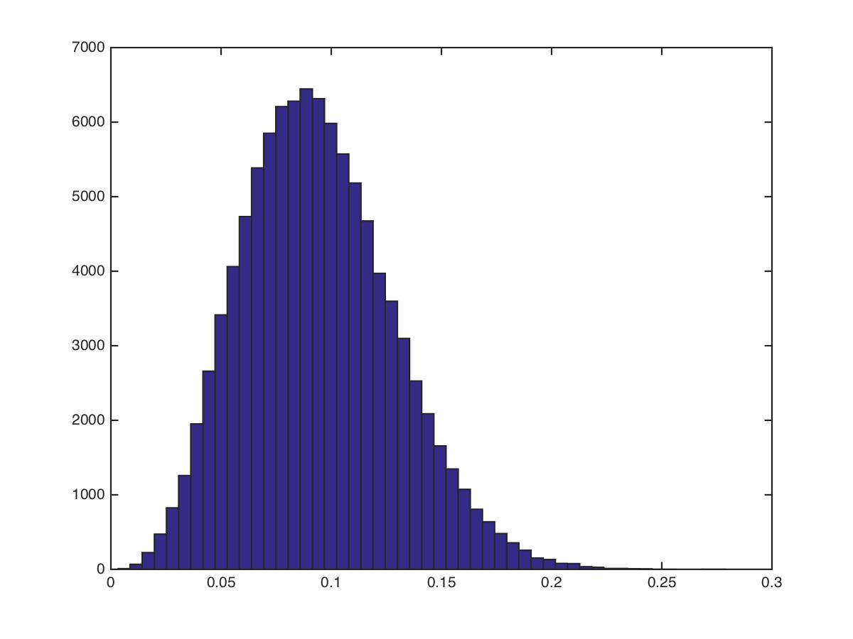
endWe can call the function like so:
>> tic; out=myfunction(1e5); toc
Elapsed time is 7.873669 seconds.
>> hist(out,50)
which produces the figure shown here:
To compile our MATLAB code into a binary MEX file we simply call the codegen function:
>> codegen myfunction -args {double(0)}The -args argument is a list of input parameters to our function myfunction and their types, which the MATLAB coder needs to know in advance, in order to produce the C code and then the binary MEX function. The double(0) just tells MATLAB that we have a single input argument that is the same type as double(0), in other words a double.
Just to unpack this a bit more—if we had a function that took two input arguments, a scalar double and a 1x10 array of doubles then we could do the following:
>> i1 = 0.0;
>> i2 = zeros(1,10);
>> codegen myfunction -args {i1, i2}
In this case we have predefined example input variables and passed those on in a cell array (hence the curly brackets).
Now if we look in our current directory we will see a binary MEX file called myfunction_mex.mexmaci64:
>> !ls -l
total 136
drwxr-xr-x  3 plg  staff    102 26 Aug 11:41 codegen
-rw-r--r--@ 1 plg  staff    126 26 Aug 11:36 myfunction.m
-rwxr-xr-x  1 plg  staff  62540 26 Aug 11:41 myfunction_mex.mexmaci64
We also see a directory called codegen that contains a subdirectory called mex and within that another directory called myfunction, that contains all of the various C files and other stuff that’s required to build the binary MEX file:
>> !ls codegen/mex/myfunction
_coder_myfunction_api.o     myfunction_initialize.c
_coder_myfunction_info.o    myfunction_initialize.h
_coder_myfunction_mex.o     myfunction_initialize.o
buildInfo.mat           myfunction_mex.mexmaci64
eml_error.c         myfunction_mex.mk
eml_error.h         myfunction_mex.mki
eml_error.o         myfunction_mex.sh
html                myfunction_mex_mex.map
interface           myfunction_terminate.c
mean.c              myfunction_terminate.h
mean.h              myfunction_terminate.o
mean.o              myfunction_types.h
myfunction.c            randn.c
myfunction.h            randn.h
myfunction.o            randn.o
myfunction_data.c       rt_nonfinite.h
myfunction_data.h       rtwtypes.h
myfunction_data.o       setEnv.sh
myfunction_emxutil.c        std.c
myfunction_emxutil.h        std.h
myfunction_emxutil.o        std.o
So now to call our compiled version of the function we just call myfunction_mex instead of calling myfunction:
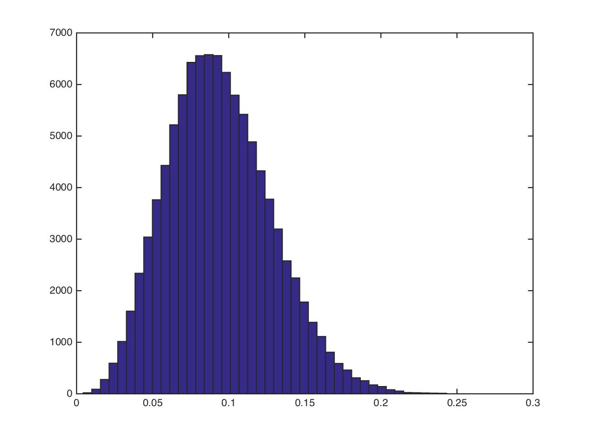
>> tic; out=myfunction_mex(1e5); toc
Elapsed time is 0.981005 seconds.
>> hist(out,50)
We can see we already achieved a significant speedup, almost 10x.
The new MEX function produces the figure shown below, which looks the same as the one produced by the plain MATLAB code, so we have some notion that our compiled MEX file is doing the right thing. Of course we should perform more stringent tests than this just to verify we are getting the expected behaviour out of the binary MEX file.
The MathWorks has a product page devoted to the Coder here:
The MathWorks also has a page on their online documentation devoted to the MATLAB Coder here: