Hanging Chain

We know from physics that a chain hung against gravity between two anchor points will adopt a curved shape known as a catenary. The cables supporting the roadways on suspension bridges like the Golden Gate bridge in San Francisco or the Lions Gate Bridge in Vancouver, adhere to this shape.

We can simulate this by modelling a chain as a sequence of N points \((x_{i},y_{i})\) for \(i=1 \ldots N\). The first (\(i=1\)) and last (\(i=N\)) points are anchors and the \(N-2\) inner points hang between the anchors, and represent the unknown parameters of the chain. What you are going to is write a MATLAB cost function to compute the potential energy of the whole chain, and then feed the free parameters (the (x,y) coordinates of the inner chain points) to a MATLAB optimizer in order to find the chain coordinates that minimize potential energy. This solution ought to correspond to a catenary shape.

Below is a textual schematic of a chain with \(N=5\) points (3 inner points and the two anchors). The outer points (x1,y1) and (x5,y5) are anchor points and are fixed in place at (x1,y1)=(0,0) and (x5,y5)=(1,0). The inner points (x2,y2), (x3,y3) and (x4,y4) are free to vary.

(x1,y1)--(x2,y2)--(x3,y3)--(x4,y4)--(x5,y5)

Click here for a MATLAB function called drawChain() that will draw a visual schematic of the chain, given input p. The input p is an array of \((2(N-2))\) points where the first \(N-2\) are the x coordinates of the \(N-2\) inner chain points, and the second \(N-2\) are the y coordinates. The code assumes that the left anchor point of the chain is fixed at (x,y)=(0,0) and the right anchor point is fixed at (x,y)=(1,0). These anchor points are not included in the input parameter p but rather are hard-coded in the function.

For example, try out this function with: drawChain([.25 .50 .75 -.1 -.2 -.1]). This corresponds to the chain points [ (0,0)–(.25,-.1)–(.50,-.2)–(.75,-.1)–(1.0,0) ].

Our modelled chain will have links between each chain point that are somewhat elastic (like rubber bands) and so the potential energy of the chain as a whole will depend on the height of the chain and on the stretch of each chain link.

The potential energy \(E\) of the chain can be computed as the sum of these two quantities:

\[E = \sum_{i=2}^{N-1} \left( m g y_{i} \right) + \sum_{i=2}^{N} \left( k \left[ L_{i} - L \right]^{2} \right)\]

where link length \(L_{i}\) is:

\[L_{i} = \sqrt{(x_{i}-x_{i-1})^{2}+(y_{i}-y_{i-1})^{2}}\]

and where \(N\) is the number of nodes in the chain, including the left and right anchor points. The value \(i=1\) corresponds to the left anchor point and the value \(i=N\) corresponds to the right anchor point.

As an exercise, write a cost function in MATLAB called chainEnergy() that takes a single parameter p as input, and produces potential energy \(E\) as output. The input parameter p should be a column vector that contains \(N\) inner chain coordinates \((x_{i},y_{i})\), with the \(x\) coordinates first followed by the \(y\) coordinates (as in drawChain above). Don’t include the left and right anchor points in p, rather hard-code them into the chainEnergy function (as in the drawChain function above).

You can assume the following values for the various chain physical parameters:

m = 0.1; % mass of each segment
g = 9.8; % gravitational constant
k = 1e2; % stiffness of each segment (inverse of stretchiness)
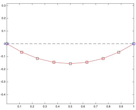
L = 0.1; % length of each segment

Optimize

Use an optimizer in MATLAB (I suggest fminunc) to solve for the (x,y) positions of a chain with 7 inner nodes (plus the two anchors) that give the lowest potential energy \(E\). Plot the result. It should look like this:

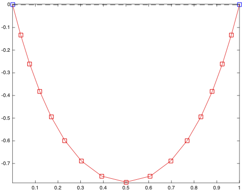
Repeat it with N=15 inner points. it should look like this:

Note: Probably a good idea to have the initial guess at the x coordinates of the inner points be monotonically increasing between 0 and 1, not totally random. The y-coordinates may be random, or maybe zero. So for example for an initial guess at \(nn\) inner chain points:

nn = 5;
x0 = linspace(0.1, 0.9, nn);
y0 = zeros(1,nn);

sample solution