Exercise 29

Local minima

Generate some (x,y) data by adapting the following MATLAB/Octave code to your language of choice:

x = 0:0.01:3;
y = sin(2*pi*x) + randn(size(x))*0.5;

Here's what the data look like (yours may look slightly different since the y values involve random values):

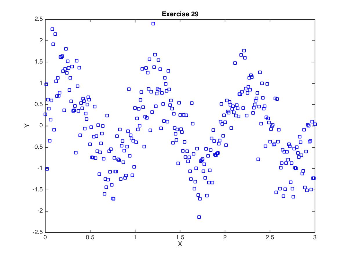
Figure 1: (x,y) data for Exercise 29

Your task is to fit a function of the following form to the data:

\begin{equation} \hat{y} = \mathrm{sin}(\beta x) \end{equation}

The (single) parameter to be optimized is \(\beta\). Your cost function \(J\) is:

\begin{equation} J = \sum_{i=1}^{n} (\hat{y_{i}} - y_{i})^{2} \end{equation}

where \(n\) is the number of \((x,y)\) pairs in the data.

Map the cost landscape

Compute the cost function \(J\) for values of \(\beta\) ranging from -10.0 to 10.0, and plot the cost landscape (plot \(J\) as a function of \(\beta\)).

Optimize for beta

Use whatever optimization method you wish, to find the value of \(\beta\) that minimizes the cost function \(J\). Plot the data and plot the best fitting function. Justify that you have found the global minimum and not a local minimum.