import numpy as np
np.random.seed(2023)
x = np.linspace(0, 7, 100)
y = np.sin(0.9040 * np.pi * x) + np.random.randn(len(x))*0.6Homework 6
Due: Mar 10 by 11:55 pm (London ON time)
Submit your Jupyter Notebook to OWL
Optimization
Generate (x,y) data:
Here’s what the data look like:
import matplotlib.pyplot as plt
plt.plot(x, y, 'o')
plt.xlabel('x')
plt.ylabel('y')
plt.show()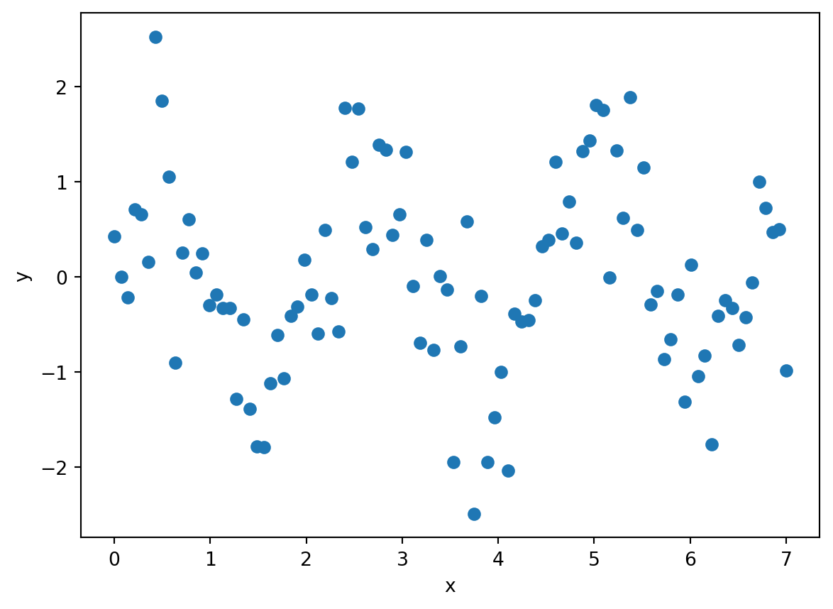
Your task is to fit a function of the following form to the data:
\[ \hat{y} = \mathrm{sin}(\beta x) \]
The (single) parameter to be optimized is \(\beta\). Your cost function \(J\) is:
\[ J = \sum_{i=1}^{n} (\hat{y_{i}} - y_{i})^{2} \]
where \(n\) is the number of \((x,y)\) pairs in the data.
Map the cost landscape
Compute the cost function \(J\) for values of \(\beta\) ranging from -5.0 to 5.0 in steps of 0.001, and plot the cost landscape (plot \(J\) as a function of \(\beta\)).
Optimize for beta
Use whatever optimization approach/method you wish, to find the value of \(\beta\) that minimizes the cost function \(J\). You can try the various methods in the scipy.optimize module or you can do something on your own (e.g. brute force grid search). If you use a gradient descent method, you should probably choose the starting guess carefully.
Plot the fit
Plot the data (\(x\) vs \(y\)) and overlay a plot of the best fitting function (\(x\) vs \(\hat{y}\)). Provide a rationale for why you think that you have found the global minimum and not a local minimum.