Plaintext Authoring
1 Why Plaintext?
- Modern Plain Text Computing by Professor of Sociology Kieran Healy
- https://plain-text.co by Kieran Healy
- Plaintext Workshop: something I put together a few years ago that presents these concepts in a more concise way, with some other examples
1.1 Scientific Documents
What does a thesis or a paper consist of, structurally?
- Sections and subsections with headings
- Body text (paragraphs of prose)
- Equations (inline and display)
- Figures with captions and cross-references
- Tables
- Citations and a bibliography
- Maybe an abstract, appendices, acknowledgements
How much of that is formatting, and how much is content?
A scientific document is structured text and data. The formatting, like fonts, margins, and line spacing, is something a template or style can handle. It’s a nuisance and a time-waster to fiddle with that stuff by hand. The principle of separation of content and style is one of the main rationales of plaintext authoring.
1.2 Word Processors
In Microsoft Word or Google Docs, content and formatting are entangled. You write a heading by selecting text and making it bold and 14pt. You don’t declare it as a heading in any structural sense (unless you use Styles, which almost nobody does consistently). The file format (.docx) is a zipped bundle of XML that is not human-readable. If Word (or Google) changes how it handles that format, or if you don’t have Word, you may not be able to open your own file in 10 years. If something goes wrong with the document you may not be able to “see” what changed because formatting and other things are hidden within menus and preferences settings.
1.3 Plaintext
In a plaintext workflow, you write your content in a simple text file, which is something you can open in Notepad, TextEdit, VS Code, or any other text editor on any computer, today or in 50 years. You mark up structure with lightweight, readable syntax (e.g. Markdown or LaTeX). Then a separate tool converts that source file into a PDF, HTML page, or even a Word document.
In the plaintext authoring model your document is:
- portable
- archivable
- version-controllable
- platform-independent
1.4 Journals
Here’s the situation:
Many journals accept LaTeX submissions directly. In physics, math, CS, and economics, LaTeX is the expected format. In neuroscience, biology, and psychology, it varies, but many journals do accept LaTeX (e.g., Nature, Nature Neuroscience, Science, PNAS, Cell, Neuron, eLife, J Neurosci, J Cogn Neurosci, all the APA journals, SAGE journals, Elsevier journals, Springer journals).
Pandoc can convert your Markdown or LaTeX source to
.docxin one command. You write in plaintext, and when a journal demands Word, you generate a Word file at the end.The real question is: where do you want to spend your time? Formatting in Word, or writing? Chasing down a reference that didn’t update, or trusting BibTeX? Emailing
thesis_v3_FINAL_revised_FINAL2.docxback and forth, or using Git?Your thesis is long. Word can struggle with documents over ~50 pages that contain many figures and cross-references.
Google Docs solves the collaboration and platform-independence problems nicely, and for short, simple documents it’s fine. But it shares Word’s limitation of entangling content and style, it has very limited equation support, it handles citations through third-party add-ons (Zotero, Paperpile), and try reformatting a 200-page Google Doc to a different journal’s style. You’ll also notice that Google Docs has no real support for cross-references, numbered equations, or figure captions that update automatically.
1.5 Summary
| Feature | Word / Google Docs | Plaintext (Markdown / LaTeX) |
|---|---|---|
| Human-readable source | No (binary/XML) | Yes |
| Version control (Git) | Difficult | Natural |
| Separation of content & style | Weak (manual) | Strong (by design) |
| Equation support | Cumbersome | Excellent (LaTeX math) |
| Citation management | Plugin-dependent | Built-in (BibTeX/CSL) |
| Long document stability | Degrades | Robust |
| Collaboration | Good (Google Docs) | Git + plain text diffs / Overleaf |
| Output flexibility | One format | PDF, HTML, Word, slides, … |
| Archival / portability | Format-dependent | Plain text lasts forever |
| Typographic quality | Acceptable | Superior (LaTeX) |
2 Markdown
Markdown is a lightweight markup language created by John Gruber in 2004. It was designed to be readable as-is. The idea is that you shouldn’t need to “compile” it to understand what the author meant.
2.1 Syntax
Here is what a Markdown document looks like:
# My Research Paper

## Introduction

This is a paragraph of text. You can make words **bold** or *italic*.
You can also include `inline code` for variable names or filenames.

Here is a list of things:

- First item
- Second item
- Third item

And a numbered list:

1. Do the experiment
2. Analyze the data
3. Write it up

## Methods

We recruited 24 participants (12 female, mean age = 22.3 years).
Stimuli were presented using PsychoPy [@peirce2019psychopy].

### Apparatus

The display was a 24-inch monitor at 60 Hz.

## Results

Reaction times are shown in Table 1 and Figure 1.
That’s it. It’s just text with some punctuation conventions.
2.2 Key Elements
| Element | Syntax | Renders as |
|---|---|---|
| Heading 1 | # Title |
Large heading |
| Heading 2 | ## Section |
Section heading |
| Heading 3 | ### Subsection |
Subsection heading |
| Bold | **bold** |
bold |
| Italic | *italic* |
italic |
| Inline code | `code` |
code |
| Link | [text](url) |
clickable link |
| Image |  |
embedded image |
| Blockquote | > quoted text |
indented quote |
| Horizontal rule | --- |
divider line |
2.3 Extensions
Pandoc (which we’ll meet next) extends basic Markdown with features essential for academic writing:
- Citations:
[@smith2020]or@smith2020 - Footnotes:
^[This is a footnote.] - Math:
$E = mc^2$for inline,$$\sum_{i=1}^n x_i$$for display - Figure captions:
{width=80%} - Tables with captions
- Cross-references (with filters like pandoc-crossref)
- YAML metadata blocks for title, author, date, and formatting options
2.4 Resources
- Markdown basics: https://www.markdownguide.org/basic-syntax/
- Pandoc’s Markdown extensions: https://pandoc.org/MANUAL.html#pandocs-markdown
- Practice: https://www.markdowntutorial.com/ (interactive, takes ~15 minutes)
3 Pandoc
Pandoc is a command-line tool created by Professor or Philosophy (and programmer) John MacFarlane. It converts between dozens of document formats, e.g.:
Markdown → PDF, Word, HTML, LaTeX (and back)
3.1 Installation
- macOS:
brew install pandoc(via Homebrew) or download from https://pandoc.org/installing.html - Windows (WSL/Ubuntu):
sudo apt install pandoc - Or download the latest release directly: https://github.com/jgc/pandoc/releases → actually: https://github.com/jgc/pandoc/releases — use https://pandoc.org/installing.html
You also need a LaTeX distribution for PDF output (Pandoc uses LaTeX under the hood to make PDFs):
- macOS:
brew install --cask mactexor the smallerbrew install --cask basictex - WSL/Ubuntu:
sudo apt install texlive-full(large, ~5 GB) orsudo apt install texlive-latex-recommended texlive-fonts-recommended texlive-latex-extra(smaller)
A lightweight alternative to a full LaTeX install is Tectonic, which auto-downloads only the packages it needs.
3.2 Usage
# Markdown to PDF
pandoc paper.md -o paper.pdf

# Markdown to Word
pandoc paper.md -o paper.docx

# Markdown to HTML
pandoc paper.md -o paper.html

# Markdown to LaTeX (to inspect or edit the .tex source)
pandoc paper.md -o paper.tex
Pandoc infers the output format from the file extension.
3.3 YAML Metadata
At the top of your Markdown file, you can add a YAML metadata block:
---
title: "Reaction Time Effects of Sleep Deprivation"
author: "Jane Smith"
date: "2025-01-15"
abstract: |
  We investigated the effects of 24 hours of sleep deprivation
  on simple and choice reaction times in 48 participants ...
bibliography: references.bib
csl: apa.csl
geometry: margin=1in
fontsize: 12pt
---
This tells Pandoc the title, author, which bibliography file to use, which citation style (CSL) to apply, and basic page geometry — all without touching a GUI.
3.4 Citations
Pandoc uses a .bib file (BibTeX format) for references. You can export .bib files from Zotero, Mendeley, Google Scholar, or write them by hand.
A .bib entry looks like this:
@article{smith2020sleep,
  author  = {Smith, Jane and Doe, John},
  title   = {Sleep deprivation and reaction time},
  journal = {Journal of Sleep Research},
  year    = {2020},
  volume  = {29},
  pages   = {e13045},
  doi     = {10.1111/jsr.13045}
}
In your Markdown, you cite it as [@smith2020sleep], and Pandoc replaces that with a formatted citation (e.g., “(Smith & Doe, 2020)”) and generates the bibliography automatically.
To compile with citations:
pandoc paper.md --citeproc -o paper.pdfThe --citeproc flag tells Pandoc to process citations. The citation style is controlled by the csl: field in your YAML header. You can download thousands of CSL styles from https://www.zotero.org/styles (APA, Vancouver, Harvard, Nature, IEEE, etc.).
3.5 Resources
- Pandoc user’s guide: https://pandoc.org/MANUAL.html
- Pandoc getting started: https://pandoc.org/getting-started.html
- Citation Style Language styles: https://www.zotero.org/styles
- BibTeX entry types: https://www.bibtex.com/e/entry-types/
3.6 Exercise 1
3.6.1 Setup
Make sure you have Pandoc and a LaTeX distribution installed (see above).
Download the files/plaintext-exercises.tgz archive, move it to your Psych_9040/ directory, and then unpack it:
$ tar -xvzf plaintext-exercises.tgzThis is what it looks like:
$ tree -F plaintext-exercisesplaintext-exercises/
├── exercise1/
│ ├── exercise1.md
│ ├── refs.bib
│ └── TASKS.md
├── exercise2/
│ ├── exercise2.tex
│ ├── refs.bib
│ ├── sample_figure.pdf
│ ├── sample_figure.png
│ └── TASKS.md
├── exercise3/
│ ├── exercise3.md
│ ├── refs.bib
│ ├── search_figure.pdf
│ ├── search_figure.png
│ └── TASKS.md
├── README.md
└── setup.shNow run the setup.sh script which downloads a .csl file that will be used for APA-style citations:
$ bash setup.shDownloading APA 7th edition citation style...
Copying apa.csl into exercise folders...
→ exercise1/apa.csl
→ exercise2/apa.csl
→ exercise3/apa.csl
Done! You're ready for the exercises.For this exercise we will be using the files in the exercise1/ directory:
3.6.2 Task
You are given a starter file exercise1.md (see below). Your tasks:
- Read the file in a text editor. Notice how readable it is even as raw text.
- Compile it to PDF:
pandoc exercise1.md --citeproc -o exercise1.pdf - Compile it to Word:
pandoc exercise1.md --citeproc -o exercise1.docx - Open both outputs. Compare them to the source.
- Add the following to the document:
- A new subsection under Methods called
### Data Analysis - A sentence describing the analysis, citing a new reference (add it to the
.bibfile) - An inline equation: the formula for a t-statistic, t = \frac{\bar{X} - \mu}{s / \sqrt{n}}
- Recompile to PDF and verify your additions appear correctly.
- A new subsection under Methods called
Hint: writing equations in LaTeX can be strange at first, they have a syntax/grammar all their own, but once you get the hang of it, it’s actually pretty easy and very efficient. Here is some documentation: LaTeX Mathematics.
3.6.3 Starter File
exercise1.md
---
title: "Effects of Caffeine on Grip Strength"
author: "A. Student"
date: "2025-02-01"
bibliography: refs.bib
csl: apa.csl
geometry: margin=1in
fontsize: 12pt
---

# Introduction

Caffeine is the most widely consumed psychoactive substance in the
world [@fredholm1999actions]. Its effects on cognitive performance
are well-documented, but effects on motor performance are less clear.

# Methods

## Participants

We recruited 30 healthy adults (15 female, mean age = 23.1 years,
SD = 3.4) from the university community.

## Procedure

Participants completed a maximal grip strength test using a hand
dynamometer before and 45 minutes after consuming either 200 mg
caffeine or placebo in a double-blind design.

# Results

Mean grip strength increased by 2.3 N (SD = 4.1) in the caffeine
condition and 0.4 N (SD = 3.8) in the placebo condition.

# Discussion

These preliminary results suggest a small positive effect of caffeine
on grip strength, consistent with @warren2010effect.

# References
3.6.4 Starter File: refs.bib
@article{fredholm1999actions,
  author  = {Fredholm, Bertil B and Bättig, Karl and Holmén, Janet
             and Nehlig, Astrid and Zvartau, Edwin E},
  title   = {Actions of caffeine in the brain with special reference
             to factors that contribute to its widespread use},
  journal = {Pharmacological Reviews},
  year    = {1999},
  volume  = {51},
  number  = {1},
  pages   = {83--133}
}

@article{warren2010effect,
  author  = {Warren, Gregory L and Park, Nicole D and Maresca,
             Robert D and McKibans, Kimberly I and Millard-Stafford,
             Mindy L},
  title   = {Effect of caffeine ingestion on muscular strength and
             endurance},
  journal = {Medicine and Science in Sports and Exercise},
  year    = {2010},
  volume  = {42},
  number  = {7},
  pages   = {1375--1387}
}
3.6.5 Debrief
- How does the PDF compare to the Word output?
- How easy is it to add a citation compared to using a Word plugin?
- What happens when you make a typo in the citation key?
3.7 Summary
We learned about:
- Why plaintext is a compelling choice for scientific writing
- The basics of Markdown syntax
- How Pandoc converts Markdown to PDF, Word, and other formats
- How to handle citations with BibTeX and CSL
In the next section we will dive into LaTeX, which is the typesetting system that pandoc uses under the hood. We will look at how to write LaTeX directly (useful for when you need fine-grained control), how to handle equations, figures, tables, and cross-references, and how to use Overleaf for collaborative LaTeX editing. Many people write LaTeX directly, bypassing Markdown and Pandoc altogether. Historical note: I wrote my very first journal article in LaTeX back in 1994, and today it is still viewable, editable, and compiles to pdf, using free and open source tools.
For next time:
- Verify that your LaTeX distribution is working: try
pdflatex --versionin your terminal. - Create a free account on Overleaf, we will use it for an exercise.
- (Optional) Work through the interactive Markdown tutorial: https://www.markdowntutorial.com/
4 Quarto
Quarto is an open-source publishing system built by Posit (the company behind RStudio). It builds on top of Pandoc but adds a layer of features that make it especially appealing for scientific writing.
Why might you care, given that you already know Markdown + Pandoc and LaTeX?
Quarto lets you embed executable code (R, Python, Julia) directly in your document. When you render the document, the code runs, and the output — figures, tables, statistical results — is inserted automatically. This means your paper and your analysis live in the same file. If your data changes, you re-render and everything updates. No more copying and pasting numbers from R into your manuscript and hoping you didn’t transpose a digit.
Beyond that, Quarto gives you cross-references, numbered figures and equations, callout blocks, and multi-format output (PDF, HTML, Word, slides, websites, books) with less configuration than raw Pandoc. It uses the same Markdown syntax you already know, with the same YAML headers and the same LaTeX math. In fact, the course notes you’re reading right now were written in Quarto markdown.
Think of it as Markdown + Pandoc with even more functionality. You get reproducible computation, richer document features, and a single tool that handles everything from a homework assignment to a thesis to a lab website, even slides for a talk.
Another example: my undergraduate course Statistics For Psychology II is done in Quarto… including the course website, the course notes, the slides, and the homeworks. The midterm and final exams are done in LaTeX.
4.1 Quarto Resources
- Quarto home: https://quarto.org/
- Getting started guide: https://quarto.org/docs/get-started/
- Gallery of examples: https://quarto.org/docs/gallery/
5 LaTeX
- TeXLive : download LaTeX
5.1 What/Why?
LaTeX (pronounced “LAH-tek” or “LAY-tek”) is a typesetting system created by Leslie Lamport in 1984, built on top of Donald Knuth’s TeX (1978). Knuth, a computer scientist, created TeX because he was unhappy with the typographic quality of his textbooks. LaTeX adds a layer of convenience on top of TeX.
When you compile a LaTeX document, the system makes thousands of micro-decisions about line breaks, hyphenation, spacing, and page layout. The result is typographically excellent output, the kind of polished, professional look you see in textbooks and journal articles.
Word processors like Microsoft Word, or Google Docs, or Apple’s Pages, are written to make some typographic “decisions” but the truth is that they pale in comparison to the polished professional look you get using LaTeX.
The benefits of LaTeX go beyond typography. Because your document is a plaintext file, you get all the advantages of plaintext authoring we discussed earlier. Your source is human-readable, and version-controllable with Git — you can see exactly what changed between drafts, roll back mistakes, and maintain a complete history of your writing without resorting to thesis_v7_FINAL_really_final.docx. The file will open in any text editor on any operating system, today or decades from now, with no dependence on a particular vendor’s software. Content and style are cleanly separated: you write \section{Methods} and a style file or document class handles how that section looks, which means you can reformat an entire document for a different journal by swapping one line in the preamble. And because LaTeX is open-source and has been in continuous use since the 1980s, there is an enormous ecosystem of packages, templates, and community support behind it.
5.1.1 Pandoc & LaTeX
When you ran pandoc paper.md -o paper.pdf above, Pandoc actually:
- Converted your Markdown to LaTeX behind the scenes
- Called
pdflatex(orxelatex) to compile the LaTeX to PDF
So you’ve already been using LaTeX. You just had Pandoc as a middleman. Learning LaTeX directly gives you much finer control when you need it. It also removes one layer of dependency/complexity from the process.
5.1.2 Which one?
| Scenario | Recommendation |
|---|---|
| Short paper, simple structure | Markdown + Pandoc |
| Blog post, course notes, README | Markdown + Pandoc |
| Thesis or dissertation | LaTeX directly (or Markdown for drafting, LaTeX for final) |
| complex equations | LaTeX directly |
| precise figure placement | LaTeX directly |
| numbered figures, equations, tables | LaTeX directly |
| Journal provides a LaTeX template | LaTeX directly |
| Need Word output for a journal | Markdown + Pandoc (convert to .docx) |
| Quick first draft | Markdown + Pandoc |
Many working scientists use a hybrid: draft quickly in Markdown, then move to LaTeX when the document matures and needs fine-tuning.
However many working scientists (and other kinds of authors) just use LaTeX ; it can be as simple or as complex as you need it to be.
5.2 Document Structure
A LaTeX document has two parts: the preamble (setup and configuration) and the document body (your content).
5.2.1 A minimal example
\documentclass{article}

\begin{document}

\section*{Abstract}

An influential idea in neuroscience is that the sensory-motor system
is activated when observing the actions of others. This idea has
recently been extended to motor learning, in which observation results
in sensory-motor plasticity and behavioral changes in both motor and
somatosensory domains. However, it is unclear how the brain maps
visual information onto motor circuits for learning. Here we test the
idea that the somatosensory system, and specifically primary
somatosensory cortex (S1), plays a role in motor learning by
observing. In experiment 1, we applied stimulation to the median nerve
to occupy the somatosensory system with unrelated inputs while
participants observed a tutor learning to reach in a force
field. Stimulation disrupted motor learning by observing in a
limb-specific manner. Stimulation delivered to the right arm (the same
arm used by the tutor) disrupted learning, whereas left arm
stimulation did not. This is consistent with the idea that a
somatosensory representation of the observed effector must be
available during observation for learning to occur. In experiment 2,
we assessed S1 cortical processing before and after observation by
measuring somatosensory evoked potentials (SEPs) associated with
median nerve stimulation. SEP amplitudes increased only for
participants who observed learning. Moreover, SEPs increased more for
participants who exhibited greater motor learning following
observation. Taken together, these findings support the idea that
motor learning by observing relies on functional plasticity in S1. We
propose that visual signals about the movements of others are mapped
onto motor circuits for learning via the somatosensory system.

\end{document}
Paste the above into an empty plaintext file, save it as simple.tex and compile it to pdf using pdflatex simple.tex. Open simple.pdf and see what it looks like.
Let’s say we want to not indent the first line of the paragraph: change the first line of the paragraph to:
\noindent An influential idea in neuroscience is that the sensory-motor systemRe-compile to .pdf and see what it looks like.
We can also specify this globally in the document by putting a command in the preamble, which is the part of the file between the documentclass command and the begin{document} command:
\documentclass{article}

\setlength{\parindent}{0pt}

\begin{document}
...
We can add another command to remove the page number from the bottom of the page:
\documentclass{article}

\setlength{\parindent}{0pt}
\pagestyle{empty}

\begin{document}
...
Re-compile and see what the .pdf looks like.
If we want left-justified (instead of full-justified text) then we can put another command in the preamble:
\documentclass{article}

\setlength{\parindent}{0pt}
\pagestyle{empty}
\raggedright

\begin{document}
...
Finally if we want 12pt font, and we want Times instead of the default LaTeX font (which is called Computer Modern):
\documentclass[12pt]{article}

\setlength{\parindent}{0pt}
\pagestyle{empty}
\usepackage{mathptmx}

\begin{document}
...
Re-compile to .pdf and see how things look.
You can see how the style gets put in one place and the content (and the semantics, like headings) remains, on its own, in the body of the document.
5.2.2 A More worked Example
\documentclass[11pt]{article}

% --- Preamble: load packages and configure ---
\usepackage[margin=1in]{geometry}
\usepackage{amsmath}          % better equation support
\usepackage{graphicx}         % for including figures
\usepackage{booktabs}         % for professional tables
\usepackage[
  backend=biber,
  style=apa,
  natbib=true
]{biblatex}                   % citation management
\addbibresource{refs.bib}

\title{Effects of Caffeine on Grip Strength}
\author{A.\ Student}
\date{February 2025}

% --- Document body ---
\begin{document}
\maketitle

\begin{abstract}
We investigated the effect of 200\,mg caffeine on maximal
grip strength in a double-blind placebo-controlled design.
\end{abstract}

\section{Introduction}

Caffeine is the most widely consumed psychoactive substance
in the world \citep{fredholm1999actions}. Its effects on
cognitive performance are well-documented, but effects on
motor performance are less clear.

\section{Methods}

\subsection{Participants}

We recruited 30 healthy adults (15 female, mean age = 23.1
years, SD = 3.4) from the university community.

\subsection{Procedure}

Participants completed a maximal grip strength test before
and 45 minutes after consuming caffeine or placebo.

\section{Results}

The results are presented in Table~\ref{tab:results} and
Figure~\ref{fig:grip}.

\section{Discussion}

These preliminary results suggest a small positive effect
of caffeine on grip strength \citep{warren2010effect}.

\printbibliography

\end{document}
I’ll admit the aesthetics of this default styling isn’t great but you can change that easily enough.
5.2.3 Key Concepts
Commands start with a backslash: \section{...}, \textbf{...}, \citep{...}
Environments are blocks delimited by \begin{...} and \end{...}: \begin{abstract}...\end{abstract}, \begin{figure}...\end{figure}
Packages extend LaTeX’s capabilities. You load them in the preamble with \usepackage{...}. It’s a similar idea to Python libraries.
Comments start with % and are ignored by the compiler.
Citations : Note that the above example uses biblatex (and the biber tool) instead of bibtex ; biblatex is just another bibliography tool that can be used with LaTeX, and it has more default styles than bibtex (https://www.overleaf.com/learn/latex/Biblatex_bibliography_styles)
5.2.4 Compiling
# Basic compilation
pdflatex paper.tex

# With bibliography (requires multiple passes)
pdflatex paper.tex
biber paper
pdflatex paper.tex
pdflatex paper.tex

# Or use latexmk, which automates the multiple passes:
latexmk -pdf paper.tex
The multiple passes are needed because LaTeX resolves cross-references and citations iteratively. latexmk handles this automatically and is the recommended way to compile.
5.3 Equations
This is where LaTeX truly shines. The equation syntax is the same whether you’re writing in LaTeX or in Markdown+Pandoc (because Pandoc passes math through to LaTeX).
5.3.1 Inline Math
Surround with single dollar signs:
The sample mean is $\bar{x} = \frac{1}{n}\sum_{i=1}^{n} x_i$.5.3.2 Display Math
Use the equation environment for numbered equations:
\begin{equation}
  t = \frac{\bar{X} - \mu_0}{s / \sqrt{n}}
  \label{eq:ttest}
\end{equation}
You can then refer to it with Equation~\ref{eq:ttest}.
For unnumbered equations use \[ and \] brackets:
\[
  \chi^2 = \sum \frac{(O_i - E_i)^2}{E_i}
\]
5.3.3 Multi-Line Equations
\begin{align}
  \text{SS}_{\text{total}} &= \text{SS}_{\text{between}}
                              + \text{SS}_{\text{within}} \\
  F &= \frac{\text{MS}_{\text{between}}}
             {\text{MS}_{\text{within}}}
\end{align}
5.3.4 Quick Reference
| What you want | LaTeX code | Renders as |
|---|---|---|
| Greek letters | \alpha, \beta, \mu, \sigma |
α, β, μ, σ |
| Subscript | x_{i} |
xᵢ |
| Superscript | x^{2} |
x² |
| Fraction | \frac{a}{b} |
a/b (stacked) |
| Square root | \sqrt{n} |
√n |
| Sum | \sum_{i=1}^{n} |
Σ |
| Integral | \int_{0}^{\infty} |
∫ |
| Hat/bar | \hat{\beta}, \bar{x} |
β̂, x̄ |
| Approximately | \approx |
≈ |
| Less/greater or equal | \leq, \geq |
≤, ≥ |
| Partial derivative | \frac{\partial f}{\partial x} |
∂f/∂x |
5.3.5 Resources
- Detexify — draw a symbol and it tells you the LaTeX code: https://detexify.kirelabs.org/
- LaTeX math cheat sheet: https://katex.org/docs/supported
- The
amsmathpackage documentation covers everything: https://mirrors.ctan.org/macros/latex/required/amsmath/amsldoc.pdf
5.4 Figures & Tables
5.4.1 Figures
\begin{figure}[htbp]
  \centering
  \includegraphics[width=0.8\textwidth]{figures/grip_strength.pdf}
  \caption{Mean grip strength (N) by condition. Error bars show
           $\pm 1$ SE.}
  \label{fig:grip}
\end{figure}
Key points:
[htbp]= placement preference: here, top of page, bottom, separate page. LaTeX decides the best placement. (This is a feature, not a bug; LaTeX optimizes page layout globally.)- Use PDF or PNG for figures. PDF is preferred for vector graphics (plots), PNG for raster images (e.g. photos, microscopy).
- Reference with
Figure~\ref{fig:grip}; the number updates automatically. - The tilde
~prevents a line break between “Figure” and the number.
5.4.2 Tables
\begin{table}[htbp]
  \centering
  \caption{Mean grip strength (N) by condition and time point.}
  \label{tab:results}
  \begin{tabular}{lcc}
    \toprule
    Condition & Pre & Post \\
    \midrule
    Caffeine  & 38.2 (5.1) & 40.5 (5.3) \\
    Placebo   & 37.9 (4.8) & 38.3 (5.0) \\
    \bottomrule
  \end{tabular}
\end{table}
Key points:
{lcc}= three columns: left-aligned, center, center.\toprule,\midrule,\bottomrulecome from thebooktabspackage and produce clean, professional horizontal rules (no vertical lines — this is a typographic best practice).- Reference with
Table~\ref{tab:results}.
Pandoc Markdown tables are simpler but less flexible:
| Condition | Pre        | Post       |
|-----------|------------|------------|
| Caffeine  | 38.2 (5.1) | 40.5 (5.3) |
| Placebo   | 37.9 (4.8) | 38.3 (5.0) |

: Mean grip strength (N) by condition and time point. {#tbl:results}
5.5 Exercise 2
In this exercise you will practice building a LaTeX document.
Make sure you have completed the setup described in Section 3.6.
For this exercise we will be using the files in the exercise2/ directory:
5.5.1 Option A: Overleaf
(Recommended for First-Timers)
- Go to https://www.overleaf.com/ and log in.
- Create a new blank project.
- Start with the minimal template from Section 5.2.2 above.
- Complete these tasks:
Task 1 — Equations: Add a “Data Analysis” subsection under Methods. Include the formula for Pearson’s correlation coefficient as a numbered equation:
r = \frac{\sum_{i=1}^n (x_i - \bar{x})(y_i - \bar{y})}{\sqrt{\sum_{i=1}^n (x_i - \bar{x})^2 \sum_{i=1}^n (y_i - \bar{y})^2}}
Then reference it in the text (“… as shown in Equation 1”).
Task 2 — Table: Add a Results table with three columns (Measure, Caffeine, Placebo) and at least two rows. Use booktabs rules. Add a caption and label, and reference the table in the text.
Task 3 — Figure: Download any plot image (or use a placeholder) and include it as a figure with a caption. Reference it in the text. (On Overleaf, use the upload button to add an image file.)
Task 4 — Citation: Add a new entry to refs.bib and cite it somewhere in the text. Verify it appears in the bibliography.
5.5.2 Option B: Locally
Same tasks, but compile locally:
latexmk -pdf exercise2.texIf you don’t have latexmk, use:
pdflatex exercise2.tex
biber exercise2
pdflatex exercise2.tex
pdflatex exercise2.tex
5.5.3 Debrief
- How did the equation-writing experience compare to Word’s equation editor?
- What happened when you changed the placement hint on your figure from
[h]to[t]? - How did adding a citation and recompiling feel compared to managing references in a GUI?
5.6 Overleaf
Overleaf deserves special mention because it addresses the most common objection to LaTeX: collaboration. Overleas is a collaborative LaTeX in the browser much like Google Docs.
- Real-time collaboration like Google Docs — multiple people can edit simultaneously
- No local installation required — everything compiles in the cloud
- Rich library of templates for journals, theses, CVs, posters: https://www.overleaf.com/latex/templates
- Git integration on paid plans — you can push/pull your Overleaf project to a Git repo
- Track changes and comments — familiar to Word users
- Free tier is generous for individual use; paid plans add more collaborators
Many universities provide institutional Overleaf subscriptions. Unfortunately at present Western does not.
For students who may not write LaTeX daily, Overleaf significantly lowers the barrier to entry. You get the typographic quality and structural rigor of LaTeX with a Google Docs-like editing experience.
5.7 A Workflow
Here are three practical workflows you might adopt:
5.7.1 Workflow 1: Markdown + Pandoc (Simplest)
Best for: drafts, short papers, course assignments, people who want minimal setup.
paper.md + refs.bib → pandoc → paper.pdf or paper.docx5.7.2 Workflow 2: LaTeX on Overleaf (Collaborative)
Best for: thesis chapters, papers with co-authors, when a journal provides a LaTeX template.
paper.tex + refs.bib → Overleaf (cloud) → paper.pdf5.7.3 Workflow 3: LaTeX Locally with Git (Maximum Control)
Best for: advanced users, large projects, integration with data analysis pipelines.
paper.tex + refs.bib → latexmk → paper.pdf
         ↑
    version controlled with Git
5.7.4 Workflow 4: Hybrid (Common in Practice)
Draft in Markdown (fast, low friction), then convert to LaTeX when the paper matures and you need fine-tuned formatting or a journal template.
draft.md → pandoc → paper.tex → edit in LaTeX → paper.pdfAll four approaches keep your source as plaintext. All four let you use Git. All four separate content from presentation.
5.8 Exercise 3
A Full Pipeline
5.8.1 Task
From a Markdown draft to polished output documents.
You are given a Markdown file representing a short paper. Your tasks:
- Compile to PDF with Pandoc. Inspect the output.
- Compile to Word with Pandoc. Open in Word. Confirm it looks reasonable.
- Compile to LaTeX with
pandoc exercise3.md -o exercise3.tex. Open the.texfile and look at what Pandoc generated. - Edit the
.texfile: adjust figure placement, tweak table formatting, or add a LaTeX-specific feature like\pagebreak. - Compile the edited
.texto PDF:latexmk -pdf exercise3.tex
5.8.2 Starter File
exercise3.md
---
title: "Visual Search Asymmetry in Threat Detection"
author: "A. Student"
date: "2025-02-15"
abstract: |
  We tested whether threatening stimuli (snakes) are detected
  faster than non-threatening stimuli (flowers) in a visual
  search task. Results supported the threat superiority effect.
bibliography: refs3.bib
csl: apa.csl
geometry: margin=1in
fontsize: 12pt
---

# Introduction

The threat superiority effect refers to the faster detection of
threatening stimuli in visual search [@ohman2001fears]. This has
been demonstrated for snakes [@ohman2001fears], spiders
[@rakison2009does], and angry faces [@fox2000facial].

# Methods

## Participants

Forty undergraduate students (28 female, mean age = 19.8,
SD = 1.2) participated for course credit.

## Stimuli and Design

Search displays contained 8 items arranged in a circle. On
target-present trials, one item was the target (snake or flower)
among 7 distractors (mushrooms). We used a 2 (target: snake,
flower) × 2 (target presence: present, absent) design.

## Data Analysis

Reaction times shorter than 200 ms or longer than 2000 ms were
excluded (1.8% of trials). We computed mean RTs for correct
responses and analyzed them with a repeated-measures ANOVA:

$$F = \frac{MS_{between}}{MS_{within}}$$

# Results

Mean reaction times are shown in Table 1.

| Target  | Present     | Absent      |
|---------|-------------|-------------|
| Snake   | 612 (89)    | 831 (102)   |
| Flower  | 698 (94)    | 854 (110)   |

: Mean reaction times in ms (SD in parentheses). {#tbl:rts}

There was a significant main effect of target type,
$F(1, 39) = 14.2$, $p < .001$, $\eta_p^2 = .27$.

# Discussion

Our findings replicate the threat superiority effect
[@ohman2001fears]. Snake targets were detected approximately
86 ms faster than flower targets.

# References
5.8.3 Debrief
- You just went from one source file to three output formats in about 60 seconds of terminal commands.
- You then had the option to “eject” to LaTeX for fine-tuning. No information was lost.
- Ask yourself: what would it be like to do this in MS Word?
5.9 Custom Style Files
Remember the principle from the beginning: separate content from style. LaTeX lets you take this even further with custom style files (.sty).
All those \usepackage commands and configuration lines in your preamble? You can move them into a .sty file and load the whole thing with a single line. For example, suppose your preamble has:
\usepackage[margin=1in]{geometry}
\usepackage{amsmath}
\usepackage{graphicx}
\usepackage{booktabs}
\usepackage[backend=biber, style=apa, natbib=true]{biblatex}
\addbibresource{refs.bib}
\usepackage{setspace}
\doublespacing
\usepackage{lineno}
\linenumbers
You can put all of that into a file called manuscript.sty:
% manuscript.sty — double-spaced, line-numbered, for journal submission
\ProvidesPackage{manuscript}

\RequirePackage[margin=1in]{geometry}
\RequirePackage{amsmath}
\RequirePackage{graphicx}
\RequirePackage{booktabs}
\RequirePackage[backend=biber, style=apa, natbib=true]{biblatex}
\addbibresource{refs.bib}
\RequirePackage{setspace}
\doublespacing
\RequirePackage{lineno}
\linenumbers
Then your .tex file’s preamble shrinks to:
\documentclass[12pt]{article}
\usepackage{manuscript}

\title{Effects of Caffeine on Grip Strength}
\author{A.\ Student}
\date{February 2025}

\begin{document}
...
Now make a second style file called preprint.sty that uses single spacing, no line numbers, and a different margin:
% preprint.sty — clean single-spaced format for preprint servers
\ProvidesPackage{preprint}

\RequirePackage[margin=1.25in]{geometry}
\RequirePackage{amsmath}
\RequirePackage{graphicx}
\RequirePackage{booktabs}
\RequirePackage[backend=biber, style=apa, natbib=true]{biblatex}
\addbibresource{refs.bib}
To switch between submission and preprint formatting, you change one line:
\usepackage{manuscript}   % for journal submission
% \usepackage{preprint}   % for preprint/sharing
Your content doesn’t change at all. The same .tex file produces a double-spaced, line-numbered manuscript for the journal, or a clean single-spaced preprint, depending on which .sty file you load. This is separation of content and style in practice.
A few notes:
- Inside
.styfiles, use\RequirePackageinstead of\usepackage. They do the same thing, but\RequirePackageis the convention for package and style files. - The
\ProvidesPackage{name}line should match the filename (without.sty). - Keep the
.styfiles in the same directory as your.texfile (or in your local texmf tree if you want them available globally). - Journal-provided LaTeX templates work on exactly this principle — they give you a
.clsor.styfile that handles all the formatting, and you just write your content.
5.9.1 Example: A Paper
Download and unpack the archive example_paper.tgz
$ tar -xvzf example_paper.tgz$ tree example_paperexample_paper
├── Figure1.pdf
├── Figure2.pdf
├── Figure3.pdf
├── Figure4.pdf
├── Figure5.pdf
├── Figure6.pdf
├── Figure7.pdf
├── jneurophysiol.bst
├── paper.tex
├── plg_jnp.sty
├── plg_min.sty
├── plg_nice.sty
└── refs.bib
1 directory, 12 filesThere is a manuscript file paper.tex, a bibtex file refs.bib, 7 Figures (Figure*.pdf), and three .sty files, which I’ve created, which styles the manuscript three different ways. The jneurophysiol.bst file is provided for us and styles the bibliography according to the J Neurophysiol style.
Open the paper.tex main manuscript file and you will see:
\documentclass{article}

% MINIMAL LATEX
\usepackage{plg_min}

% IMPROVED LATEX
% \usepackage{plg_nice}

% MY "J Neurophysiol classic" PREPRINT STYLE
% \usepackage{plg_jnp}


\title{A Context-Free Model of Savings in Motor Learning}

\author[1,$\ddagger$]{Mahdiyar Shahbazi}
\author[2,3]{Olivier Codol}
\author[4,5,$\dagger$]{Jonathan A. Michaels}
\author[1,4,$\dagger$,*]{Paul L. Gribble}
\affil[1]{Dept. Psychology, Western University, London, ON, Canada}
\affil[2]{Mila--Qu\'ebec Artificial Intelligence Institute, Montr\'eal, QC, Canada}
\affil[3]{Dept. Neuroscience, Universit\'e de Montr\'eal, Montr\'eal, QC, Canada}
\affil[4]{Dept. Physiology \& Pharmacology, Schulich School of Medicine \& Dentistry, London, ON, Canada}
\affil[5]{School of Kinesiology and Health Science, Faculty of Health, York University, Toronto, ON, Canada}
\affil[$\dagger$]{Co-senior authors}
\affil[$\ddagger$]{Present address: Dept. Organismic and Evolutionary Biology, Harvard University, Boston, MA, USA}
\affil[*]{Corresponding author: [email protected]}

\date{\normalsize\today}


\begin{document}

\maketitle
\thispagestyle{empty}

\begin{abstract}
Learning to adapt voluntary movements to an external perturbation, whether mechanical or visual, is
Try compiling the document to a .pdf as it is now (with \usepackage{plg_min} uncommented):
$ pdflatex paper.tex
$ bibtex paper.tex
$ pdflatex paper.tex
$ pdflatex paper.tex
Open paper.pdf and have a look.
Now try commenting out \usepackage{plg_min} and uncommenting \usepackage{plg_nice}. Recompile to .pdf. See how it looks now.
Now try commenting out \usepackage{plg_nice} and uncommenting \usepackage{plg_jnp}. Recompile to .pdf. See how it looks now. (Note you may have to first delete all the intermediate files that were created from above. Try latexmk -c paper and then rm paper.bbl before you recompile using pdflatex and bibtex.)
The possibilities for styling a LaTeX document are almost endless. Anything you can think of, you can do.
5.9.2 Example: A Letter
As a final example, some time ago I created a LaTeX style file that duplicates the official Western letterhead, so that I could easily write letters. As a result, I can write a letter like this:
\documentclass{Psychology_letter}

\begin{document}

\thedate{\today}

\recipient{Ford Prefect\\
Arthur's friend\\
The Hitchhiker's Guide to the Galaxy}

\regarding{something important}

\greeting{Dear Colleague,}

Isn't it great to be able to write a letter using LaTeX and
not have to open MS Turd, and deal with fonts, hidden menus,
and changes in formatting, not to mention random crashes. In
addition this plaintext file will be readable forever, using
any text editor, on any operating system.

\closingsig{Sincerely,}

\end{document}
A quick compile:
$ xelatex letter.texand I get a file letter.pdf that looks like this:

Once you spend some time writing documents using LaTeX, going back and dealing with MS Turd is quite a shock to the system.
5.10 Citations using .csl
Markdown + Pandoc is able to use .csl styles from the Citation Style Language (CSL) repository … and there are hundreds available, much more than the default styles available in BibTeX or BibLaTeX. Can we use .csl styles directly with LaTeX?
The answer is a qualified yes. We have seen how we can use pdflatex to compile LaTeX documents and we can also use xelatex (for example which is necessary when using the fontspec package to have custom fonts) … but there is a third way to compile LaTeX documents, and it’s called lualatex (based on the Lua programming language).
The lualatex tool is able to compile LaTeX documents that use a .csl file to define citation/bibliography styles. Here is an example:
\documentclass[11pt]{article}
\usepackage[style=nature]{citation-style-language} % make sure nature.csl exists in the same directory
\addbibresource{refs.bib}
\usepackage{fontspec} % with fontspec, use xelatex or lualatex not pdflatex
\setmainfont{Palatino}
\setsansfont{Helvetica Neue}
\usepackage[margin=1.2in]{geometry} % define page margins
\usepackage{microtype} % makes even better typography
\usepackage{titlesec} % style section and subsection headings
\titleformat*{\section}{\bfseries\sffamily\large}
\titleformat*{\subsection}{\bfseries\sffamily\normalsize}
\usepackage{lipsum} % for generating placeholder text
\begin{document}
\title{The Answers to Important Questions}
\author{Jane Smith, Ph.D.}
\date{\today}
\maketitle
\thispagestyle{empty} % no page number on first page
\section*{Abstract}
\lipsum[1]
\section*{Introduction}
\lipsum[2]
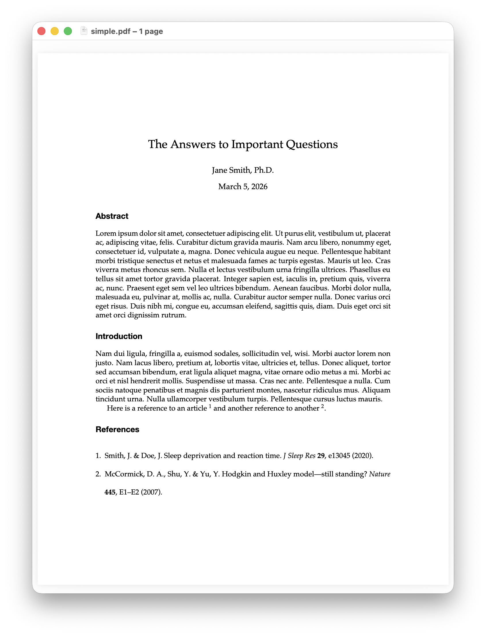
Here is a reference to an article \citep{smith2020sleep} and another reference to another \citep{mccormick2007hodgkin}.
\printbibliography
\end{document}We compile using lualatex three times (usually three is necessary to get all the references sorted):
$ lualatex simple.tex
$ lualatex simple.tex
$ lualatex simple.tex
And here is the .pdf:
The other way is to use pdflatex (or xelatex) once, then run a tool called citeproc-lua on the .aux file that’s produced by the first command (pdflatex or xelatex)… this produces the .bbl file needed for the bibliography. Then run pdflatex or xelatex again and the .pdf will be generated.
6 Quick Reference
6.1 Terminal Commands
# Pandoc: Markdown to PDF
pandoc paper.md --citeproc -o paper.pdf

# Pandoc: Markdown to Word
pandoc paper.md --citeproc -o paper.docx

# Pandoc: Markdown to LaTeX
pandoc paper.md -s -o paper.tex

# LaTeX: compile with automatic re-runs
latexmk -pdf paper.tex

# LaTeX: clean up auxiliary files
latexmk -c
6.2 Tools
| Tool | What it does | Link |
|---|---|---|
| Pandoc | Universal document converter | https://pandoc.org/ |
| TeX Live | Full LaTeX distribution (Linux/Windows) | https://tug.org/texlive/ |
| MacTeX | TeX Live for macOS | https://tug.org/mactex/ |
| Overleaf | Collaborative LaTeX editor in the browser | https://www.overleaf.com/ |
| Zotero | Reference manager (exports .bib) | https://www.zotero.org/ |
| Better BibTeX | Zotero plugin for clean .bib export | https://retorque.re/zotero-better-bibtex/ |
| Detexify | Draw a symbol → get LaTeX code | https://detexify.kirelabs.org/ |
| TeXstudio | Local LaTeX editor with preview | https://www.texstudio.org/ |
| VS Code + LaTeX Workshop | LaTeX editing in VS Code | https://marketplace.visualstudio.com/items?itemName=James-Yu.latex-workshop |
6.3 Further Learning
- Overleaf’s LaTeX tutorials (excellent for beginners): https://www.overleaf.com/learn
- The Not So Short Introduction to LaTeX2e (classic free guide): search CTAN for “lshort”
- LaTeX Wikibook: https://en.wikibooks.org/wiki/LaTeX
- Pandoc User’s Guide: https://pandoc.org/MANUAL.html
- LaTeX StackExchange (Q&A community): https://tex.stackexchange.com/
- BibTeX entry types and fields: https://www.bibtex.com/e/entry-types/
- Plaintext Workshop: something I put together a few years ago that presents these concepts in a more concise way, with some other examples