Reproducibility & Replicability II: clean code
Principles of Clean Code
1 Why
Writing small scripts to solve toy programming puzzles is one thing, but writing a large amount of inter-connected code to analyse a dataset is quite another. What’s more, organizing the data itself is something that can have a big impact on the organization and clarity of the code. It’s worth talking about and thinking about some basic principles for organizing data and code for realistic scenarios such as scientific experiments and data analysis work.
Before we get into principles, here is a cautionary tale.
A Scientist’s Nightmare: Software Problem Leads to Five Retractions
In 2007, Geoffrey Chang, a rising star in structural biology, had to retract five papers (three from Science, one from PNAS and one from J Mol Biol). The reason? A bug in a data-processing script had flipped two columns of data, inverting the electron-density map from which his team had derived protein structures. The code ran without errors. The results looked plausible. The bug hid in plain sight for years because the code was written in a way that made it very difficult for anyone, including Chang himself, to verify what it was actually doing.
This is not an isolated incident. Researchers in genomics, economics, and psychology have all experienced retractions or corrections traced back to code errors that might have been caught earlier if the code had been written more carefully.
The point is: your analysis code is a methods section. If nobody can read it, nobody can reproduce your results, and nobody, including future-you, can catch mistakes. Clean code is not about aesthetics. It is about scientific integrity.
I want you to read the following:
- Writing clean code guide from the Jörn Diedrichsen lab blog
This guide is excellent and covers a lot of ground. What follows below expands on several of its key ideas with worked examples in Python, using the kinds of data and analyses you’ve been working with this semester.
2 Naming
The single easiest thing you can do to improve your code is to name things well (variables, functions, files, directories). Good names make comments unnecessary. Bad names make even simple code confusing.
2.1 Variables
Consider this snippet:
d = np.loadtxt("data.csv", delimiter=",", skiprows=1)
x = d[:, 2]
m = np.mean(x[x < 1.5])
It runs. It produces a number. But what is d? What is column 2? What does 1.5 mean? Now compare:
grip_data = np.loadtxt("grip_strength_data.csv", delimiter=",", skiprows=1)
post_grip_force = grip_data[:, 2]
max_force_cutoff = 1.5  # exclude trials above 1.5 N/kg (equipment ceiling)
mean_force = np.mean(post_grip_force[post_grip_force < max_force_cutoff])
Same computation. But now the code tells you what it is doing. A reader does not need to cross-reference a data dictionary to figure out what column 2 contains.
Some guidelines:
- Use descriptive nouns for variables:
reaction_times,participant_ids,mean_rt_caffeine. Notd,x,m. - Be consistent: if you abbreviate “reaction time” as
rt, userteverywhere. Don’t mixrt,react_time,RT, andreaction_tin the same project. - Single-letter names are fine in small scopes:
for i in range(n_trials)is perfectly clear. A loop index does not need to be calledtrial_indexunless the loop body is very long. - Name magic numbers: if
200appears in a line of code, nobody knows why.min_rt_ms = 200makes the intent obvious.
2.2 Functions
Where variable names are nouns, function names should be verbs (or verb phrases). They should say what the function does:
| Bad | Better |
|---|---|
func1() |
load_participant_data() |
process() |
exclude_outlier_trials() |
do_stats() |
run_paired_ttest() |
my_plot() |
plot_condition_means() |
2.3 Files & directories
The same principle applies to file names:
| Bad | Better |
|---|---|
data.csv |
grip_strength_raw.csv |
analysis.py |
01_preprocess.py or analyze_grip_strength.py |
fig1.png |
figure_grip_by_condition.png |
Untitled3.py |
(delete it) 😜 |
3 Modularity
When you first start writing analysis code, the natural thing to do is to write a script: a long sequence of steps, from loading data to producing a figure, all in one file. This works fine for short tasks. But as your analysis grows, a single long script becomes hard to read, hard to debug, and hard to reuse.
The remedy is to modularize your code by breaking it up into functions, each of which does one specific thing.
3.1 A messy script
Here is a working script that analyses a small grip strength experiment. It loads data, excludes outlier trials, computes condition means for each participant, runs a paired t-test, and makes a bar chart. The code is realistic, and it produces the correct result. But it is hard to read. Go through it line by line with an eye towards trying to understand what it does (and remember, this could be your code, being read by future-you):
import numpy as np
import matplotlib.pyplot as plt
from scipy import stats

d = np.loadtxt("grip_strength_data.csv", delimiter=",", skiprows=1)
# col 0 = subj, col 1 = condition (0=placebo,1=caffeine), col 2 = force
s = np.unique(d[:, 0])
m1 = []
m2 = []
for i in s:
    tmp = d[d[:, 0] == i]
    tmp1 = tmp[tmp[:, 1] == 0]
    vals1 = tmp1[:, 2]
    vals1 = vals1[(vals1 > 5) & (vals1 < 80)]
    m1.append(np.mean(vals1))
    tmp2 = tmp[tmp[:, 1] == 1]
    vals2 = tmp2[:, 2]
    vals2 = vals2[(vals2 > 5) & (vals2 < 80)]
    m2.append(np.mean(vals2))
m1 = np.array(m1)
m2 = np.array(m2)
t, p = stats.ttest_rel(m2, m1)
print(f"t = {t:.3f}, p = {p:.3f}")
fig, ax = plt.subplots()
means = [np.mean(m1), np.mean(m2)]
sems = [stats.sem(m1), stats.sem(m2)]
ax.bar([0, 1], means, yerr=sems, capsize=5, color=["#4e79a7", "#e15759"])
ax.set_xticks([0, 1])
ax.set_xticklabels(["Placebo", "Caffeine"])
ax.set_ylabel("Grip Force (N)")
ax.set_title("Grip Strength by Condition")
plt.tight_layout()
plt.savefig("fig.png", dpi=150)
plt.show()
What’s wrong with this code? It works, but:
- Variable names like
d,s,m1,m2,tmp,tmp1,tmp2,vals1,vals2say nothing about what they contain - The magic numbers
5and80appear without explanation - The block that computes means for placebo is nearly identical to the block for caffeine (copy-paste code, a classic no-no)
- There are no functions, so nothing is reusable or independently testable
- It is 30+ lines with no structure; to understand the flow you must read every line
3.2 A clean version
Here is the same analysis, refactored. Read through it with an eye towards understanding what is happening and how it works:
import numpy as np
import matplotlib.pyplot as plt
from scipy import stats


MIN_FORCE_N =  5   # below this = no grip detected
MAX_FORCE_N = 80   # above this = equipment ceiling

CONDITION_PLACEBO  = 0
CONDITION_CAFFEINE = 1


def load_grip_data(filepath):
    """Load grip strength data from a CSV file.

    Args:
        filepath: Path to CSV with columns [subject_id, condition, force_n].

    Returns:
        NumPy array with shape (n_trials, 3).
    """
    return np.loadtxt(filepath, delimiter=",", skiprows=1)


def compute_subject_means(data, condition):
    """Compute mean grip force per subject for a given condition.

    Trials with force outside (MIN_FORCE_N, MAX_FORCE_N) are excluded.

    Args:
        data: Array with columns [subject_id, condition, force_n].
        condition: Condition code to select (0 or 1).

    Returns:
        Array of per-subject mean forces.
    """
    subject_ids = np.unique(data[:, 0])
    subject_means = np.zeros(len(subject_ids))
    for i, subj in enumerate(subject_ids):
        subj_trials = data[(data[:, 0] == subj) & (data[:, 1] == condition)]
        forces = subj_trials[:, 2]
        valid = forces[(forces > MIN_FORCE_N) & (forces < MAX_FORCE_N)]
        subject_means[i] = np.mean(valid)
    return subject_means


def plot_condition_means(means_placebo, means_caffeine, output_path):
    """Create a bar chart comparing grip force between conditions.

    Args:
        means_placebo: Array of per-subject means for placebo.
        means_caffeine: Array of per-subject means for caffeine.
        output_path: Filepath for the saved figure.
    """
    group_means = [np.mean(means_placebo), np.mean(means_caffeine)]
    group_sems = [stats.sem(means_placebo), stats.sem(means_caffeine)]

    fig, ax = plt.subplots()
    ax.bar([0, 1], group_means, yerr=group_sems, capsize=5,
           color=["#4e79a7", "#e15759"])
    ax.set_xticks([0, 1])
    ax.set_xticklabels(["Placebo", "Caffeine"])
    ax.set_ylabel("Grip Force (N)")
    ax.set_title("Grip Strength by Condition")
    plt.tight_layout()
    plt.savefig(output_path, dpi=150)
    plt.show()


# --- Main analysis ---
if __name__ == "__main__":
    grip_data = load_grip_data("grip_strength_data.csv")

    means_placebo  = compute_subject_means(grip_data, CONDITION_PLACEBO)
    means_caffeine = compute_subject_means(grip_data, CONDITION_CAFFEINE)

    t_stat, p_value = stats.ttest_rel(means_caffeine, means_placebo)
    print(f"Paired t-test: t = {t_stat:.3f}, p = {p_value:.3f}")

    plot_condition_means(means_placebo, means_caffeine, "figure_grip_by_condition.png")
What changed?
The main thing is that the overall structure of the python script changed so that we have variables with important values defined at the top, then a series of functions defined in the body, and at the bottom the if __name__ == "__main__": “main” section defined.
Recall when a Python script has a if __name__ == "__main__": section defined, that code is executed when the script is executed (e.g. from a terminal with python3 myscript.py). When the script is imported by other python code (e.g. import myscript) then the variables and functions are imported but the “main” part is not executed.
Other things that are different in the refactored code:
- Magic numbers are named constants at the top of the file. If the cutoff changes, you change one line, not two (or four, or six).
- The copy-pasted blocks are now one function (
compute_subject_means) called twice with different arguments. If you need to change the outlier logic, you change it in one place. - Each function has a docstring that says what it does, what it takes, and what it returns.
- The main analysis reads like an outline: load data, compute means, run test, make figure. You can understand the flow without reading the details of each step.
- Each function is independently testable: you could call
compute_subject_meanson a small hand-crafted array and verify it gives the right answer.
The code is longer, but it is not more complex. In fact it is less complex because the structure is explicit rather than implicit.
3.3 Key principles
- Functions should do one thing, and do it well.
- Functions should only receive the information they need
- Your top-level script should read like a table of contents: load, process, analyze, plot.
- Aim for shallow call depth: ideally you have elemental functions (do one operation), process functions (chain several elemental functions), and scripts (call process functions). Three levels is usually enough.
5 Project Organization
5.1 Data Processing Stages
It is useful to think about the life cycle of data as we move from “raw” data files all the way to publication-quality figures and statistical tests.
In data oriented scientific research we often start with one or more “raw” data files. These can be generated by pieces of laboratory equipment (e.g. EEG, fMRI, EMG, RTs from a keyboard, participant responses, etc) or they may be provided by others.
Typically there is a need to process, or filter, or slice, or perform other operations on raw data before we reach the stage where we can perform statistical analyses or plot summary figures. It is useful to think about a first stage of data processing whereby we load in raw data files and generate “processed” or “analysed” data files that store a more useful component or product of the raw data files. Often the analysed data files are much smaller (e.g. orders of magnitude smaller) than the raw data files. For example we may have 100 raw data files, one for each participant, and after filtering, slicing, and separating out the most important components, we may end up with 100 analysed data files, one for each participant, that are each 10x smaller than the raw data files.
Then there may be one or more kinds of analyses, and/or plots, that one wishes to perform, and instead of loading raw data files from scratch and performing the filtering/processing steps above, again, instead we operate directly on the analysed data files. This saves time (faster to load) and it also separates out the first stage of data processing from the second stage of summary analyses, plots, etc.
Then often we can think of a third step, whereby we want to combine or summarize the analysed data files (e.g. one per participant) into group-level analyses. Perhaps from each participant’s analysed data file, we extract key dependent measures, and collect them together, for all participants, into a single tabular file (e.g. a .csv or .tsv), what we might call a summary file. Then all statistical analyses, group-level plots, can operate directly from the summary files, without having to load the analysed files or the raw files.
One great advantage of thinking about the workflow in this way is that each stage of data analysis is kept perfectly modular, and only depends upon the data files a the level “below”. You can pass summary data to a colleague and only need to give them the code a the top level, which operates on the summary data. Code and data organized together this way is extremely portable, understandable, debuggable, and shareable.
In your own research, think about the stages of processing between raw data, intermediate data structures, and “final” data used for figures and statistical analyses.
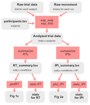
from the Writing clean code guide by Jörn Diedrichsen; go and read the section in his blog post titled “Data Structures”
It should be crystal clear how to get each Figure or statistical analysis from data + code. Jörn suggests it and I agree: write out on a piece of paper what this directed graph looks like for your paper/project.
5.2 Directory structure
Here is a sensible layout for a small research project:
grip_strength_study/
├── README.md
├── requirements.txt
├── data/
│   └── grip_strength_raw.csv
├── scripts/
│   ├── 01_preprocess.py
│   └── 02_analyze.py
├── figures/
│   └── figure_grip_by_condition.png
└── results/
    └── stats_output.txt
A few principles:
- Raw data is read-only. Never modify your original data files. If you need to preprocess, write a script that reads the raw data and writes processed data to a separate file or directory.
- Separate code from data from outputs. This makes it obvious what is source material, what is code, and what is generated.
- Include a
README.mdthat says what the project is, how to run the analysis, and what the dependencies are. - Include a
requirements.txt(orpyproject.toml) listing your Python dependencies and their version numbers, so someone else can recreate your environment. If you are usinguv, apyproject.tomlfile will be created for you.
If you end up with a large number of data files and distinct “raw”, “processed” and “summary” levels of data structures, put them in distinct directories, e.g. data/raw/, data/processed/ and data/summary/.
5.3 Code + Paper
- Code should reside in a publicly accessible repository (e.g. on GitHub)
- Each Figure and each statistical analysis should be reproducible by running a single script/function without changes
- Data should accompany the code (GitHub is not the place to store very large data files, but files at the summary level, e.g.
.csvtabular files are likely fine)
5.4 Code sharing (GitHub)
GitHub is a version control system and code-sharing platform that allows you to track changes to your code over time and collaborate with others. You can use GitHub to store and manage your code, data analysis notebooks, and even data (though not gigantic amounts of data), ensuring you can revert to previous versions if needed. GitHub works well with a number of other useful programs like Visual Studio Code and the online LaTeX document system Overleaf.
- Get Started with GitHub
- GitHub Skills
6 Exercises
6.1 Setup
Download the clean-code-exercises.tgz archive, move it to your Psych_9040/ directory, and unpack it:
$ tar -xvzf clean-code-exercises.tgzThis is what it looks like:
$ tree -F clean-code-exercisesclean-code-exercises/
├── exercise1/
│ ├── messy_analysis.py
│ ├── data/
│ │ └── rt_experiment_data.csv
│ └── TASKS.md
├── exercise2/
│ ├── analyze_data.py
│ ├── experiment_data.csv
│ ├── make_figure.py
│ ├── test.py
│ ├── Untitled1.py
│ ├── fig1.png
│ └── TASKS.md
└── README.md6.2 Exercise 1
Refactor a messy script.
Task
In the exercise1/ directory you will find a script called messy_analysis.py and a data file data/rt_experiment_data.csv. The data file contains simulated reaction time data from a visual search experiment with two conditions (feature search and conjunction search). The script loads the data, excludes outlier trials, computes per-subject condition means, runs a paired t-test, and makes a bar chart.
The script works. Run it and confirm you get a t-statistic, a p-value, and a figure.
Your task is to refactor the script so that:
- Variable names are descriptive
- Magic numbers are replaced with named constants
- Repeated code is eliminated using functions
- Each function has a Google-style docstring
- The main analysis reads like a short outline
Your refactored script must produce the same numerical output and the same figure.
Submit: your refactored .py file.
Debrief
- How many functions did you end up with?
- Which parts of the original script were hardest to clean up?
- Could someone unfamiliar with the experiment understand your refactored code without additional explanation?
6.3 Exercise 2
Organize a messy project.
Task
The exercise2/ directory contains a small “project” — a handful of scripts, a data file, and an output figure, all dumped flat in one directory. Some files are useful. Some are not. There is no README.
Examine the files and figure out what the project does. Then:
- Reorganize the project into a clean directory structure (e.g.
data/,scripts/,figures/). - Delete files that are clearly junk (scratch files, unnamed files).
- Rename files to be descriptive.
- Write a
README.mdthat describes: what this project does, what the data file contains, how to run the analysis, and what packages are needed. - Create a
requirements.txtlisting the Python dependencies. - (Optional) Initialize a git repository (
git init), add your files, and make a first commit.
Submit: your reorganized project directory (as a .zip or .tgz), including the README.
Debrief
- What directory structure did you choose and why?
- What did you put in the README?
- If you came back to this project in a year, would you know what to do?
7 Resources
- Writing clean code guide from Jörn Diedrichsen’s lab
- Better Code, Better Science by Russ Poldrack — especially the Principles of software engineering and Project structure and management chapters
- book: Clean Code: A Handbook of Agile Software Craftsmanship by Robert Martin
- a shorter book: A philosophy of software design by John Ousterhout, (and an accompanying website)
- PEP 8 — Python’s official style guide
4 Comments & Docstrings
There is a saying (I think from the Code Complete book by Steve McConnell) that good code is its own best documentation.
If you have to write very long comments to explain how your code works, it may be because your code is not very clean. Ideally, code should be self-explanatory.
4.1 When comments help
Good comments explain why, not what:
The code already says what it does (select trials with
trial_num > 5). The comment says why (they are practice trials).4.2 Unnecessary comments
This comment adds nothing. The code is already clear (well, it would be clearer if
xhad a better name).4.3 Docstrings
Every function you write for a project should have a docstring. It doesn’t need to be long. A good convention to follow is Google-style (Google Python Style Guide: Functions and Methods).
At a minimum a good docstring should contain:
Notice that with a descriptive function name and a good docstring, the function body barely needs any inline comments.