Bivariate Correlation Review

Today

Bivariate Correlation Review

• correlation vs causation
• correlation strength/direction
• Pearson’s r using cor()
• significance test using cor.test()
• random correlations & sample size

Causation

1. Hitting a ball can cause it to move

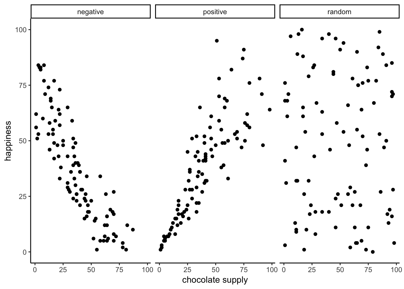
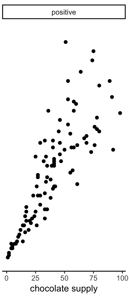
2. The action of the causal force can be measured by relating a measure of the cause (swing strength) to a measure of the outcome (distance travelled)

3. There is a positive relationship between the two measures, increasing swing strength is associated with longer distances

Correlation

4. We use the term correlation to describe the relationship between the two measures, in this case we found a positive correlation

5. We have seen that a causal force (swing strength) can produce a correlation between two measures

Causation & Correlation

1. Psychological science is interested in understanding the causes of psychological processes

2. We can measure change in a causal force (an indepdendent variable), and measure change in an outcome (psychological process, a dependent variable)

3. If the force does causally change the outcome, we expect a relationship or association between the force and the outcome (we can measure this as a correlation between the two variables)

Causation

• a causal relationship between X and Y predicts a correlation between X and Y
  • we can test whether there’s a correlation between X and Y
  • if there isn’t a correlation, that argues against a causal relationship
  • falsification of our hypothesis
• BUT the other way around doesn’t work
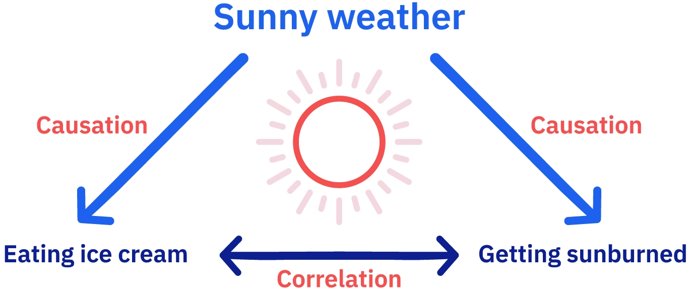
  • the observation of a correlation between X and Y does not represent evidence of a causal relationship between X and Y
  • it doesn’t prove X causes Y
  • if you conclude so, you make the classic logical error called affirming the consequent

Affirming the Consequent

• if theory T is true, that predicts data/pattern P should be seen
  • if you don’t see P, that is evidence against theory T
• if you do observe pattern P, that does not prove theory T
  • why? P could be caused by something other than T

Affirming the Consequent

• theory: I have covid-19
  • prediction: covid-19 causes a fever
  • observation: I do have a fever
  • conclusion: I have covid-19
    • LOGICAL ERROR!
• I could have a fever for many other reasons

Example:

• your hypothesis: does spending more time on social media negatively affect mental health?
• you collect data on a sample of 100 students
  • a questionnaire gives a depression rating between 1 and 10
  • they also report time spent on social media in a typical week in hours per day
• you find a correlation does exist between the two measures
  • is this evidence in support of your hypothesis?
  • NO!—LOGICAL ERROR! (affirming the consequent)

3 kinds of correlation

Positive correlation

• Increases in the X variable are associated with
  increases in the Y variable

• Decreases in the X variable are associated with
  decreases in the Y variable

Negative correlation

• Increases in the X variable are associated with
  decreases in the Y variable

• Decreases in the X variable are associated with
  increases in the Y variable

Random (no correlation)

• Increases in the X variable are NOT associated with
  increases or decreases in the Y variable

• Decreases in the X variable are NOT associated with
  increases or decreases in the Y variable

Increasing positive correlation

Negative correlations

Correlation Strength

• Super strong (Perfect): dots all line up, no exceptions
• Strong: Clear pattern, not much variation in dots
• Medium: There is a pattern but dots have a lot of variaion
• Weak: Sort of a hint of a pattern, dots have loads of variation
• None: Dots are everywhere, no clear pattern

Pearson’s r

A number that summarizes the strength & direction of a correlation

• varies between -1.0 and 1.0
• 0.0 means no correlation
• 1.0: perfect positive correlation
• -1.0: perfect negative correlation
• values in between: more or less strength

Formula for Pearson’s r

R: Pearson’s r

x <- c(1,2,3,4,5)
y <- c(4,3,6,7,8)
N <- 5
covariation<-sum((x-mean(x))*(y-mean(y)))/N
SD_x <- sqrt(sum((x-mean(x))^2)/N)
SD_y <- sqrt(sum((y-mean(y))^2)/N)
r <- covariation/(SD_x*SD_y)
r

[1] 0.9149914

R’s cor() function

R has a function to compute correlations called cor()

x <- c(1,2,3,4,5)
y <- c(4,3,6,7,8)
cor(x,y)

[1] 0.9149914

What do correlations mean?

Could mean that one variable causes change in another variable

BUT, it can mean other things…

1. Causal direction problem
2. Non-linear problem
3. Spurious correlations
4. Chance correlations
5. Third variable as cause

1 Causal Directionality problem

2 Nonlinearity problem

3 Spurious correlations

http://www.tylervigen.com/spurious-correlations

4 Chance correlations

Correlations between two datasets (samples from a population) can occur by chance, and be completlely meaningless

• we will do some simulations!

5 Third variable

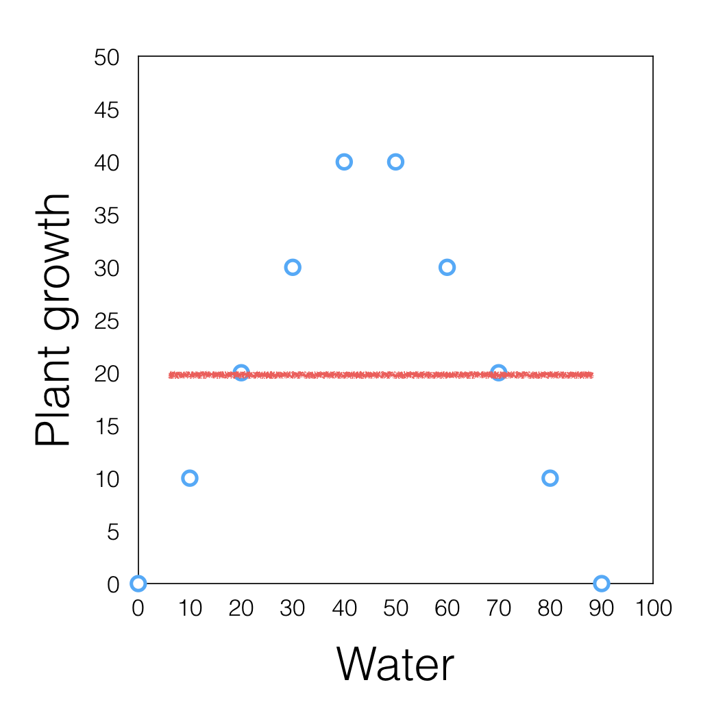
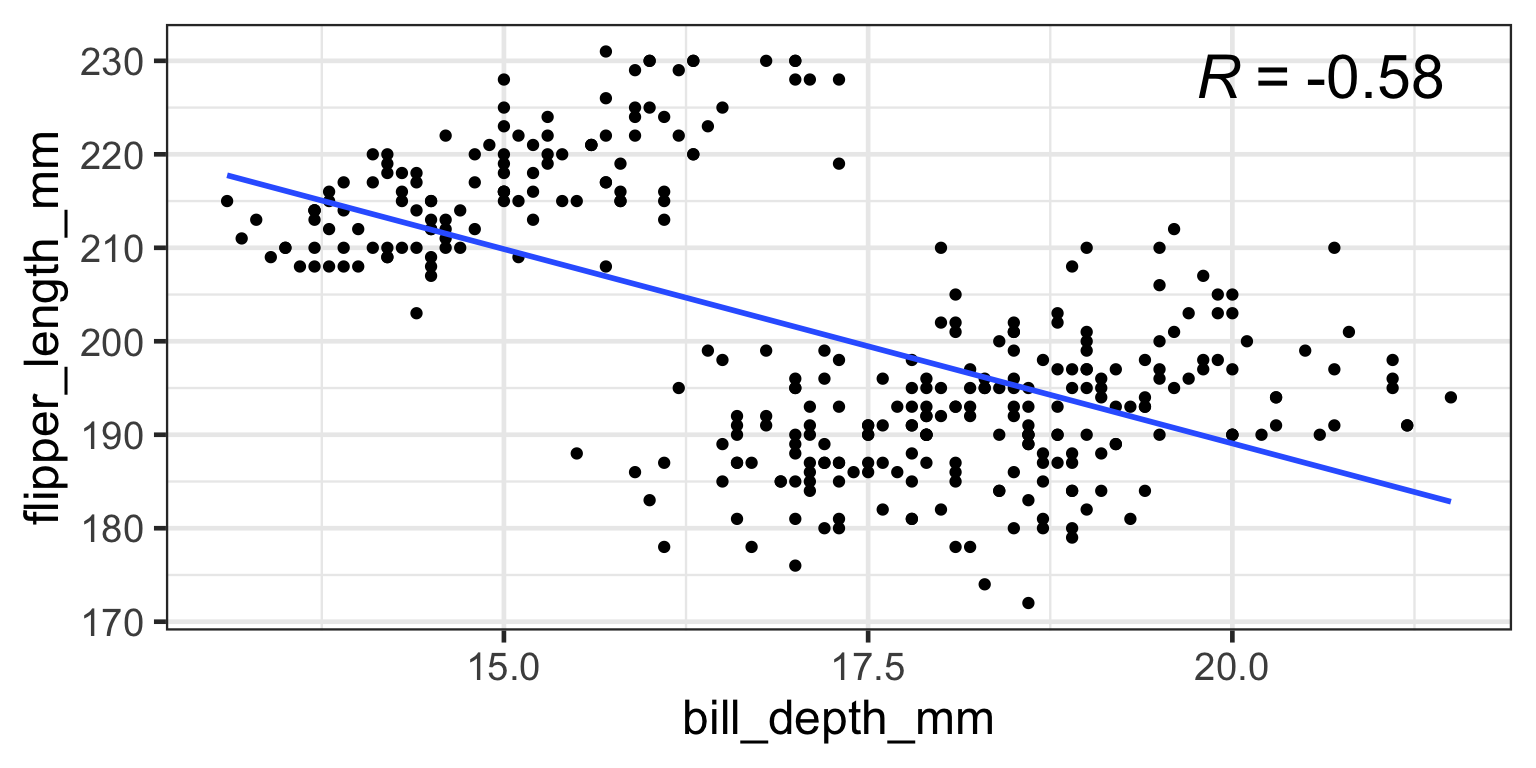
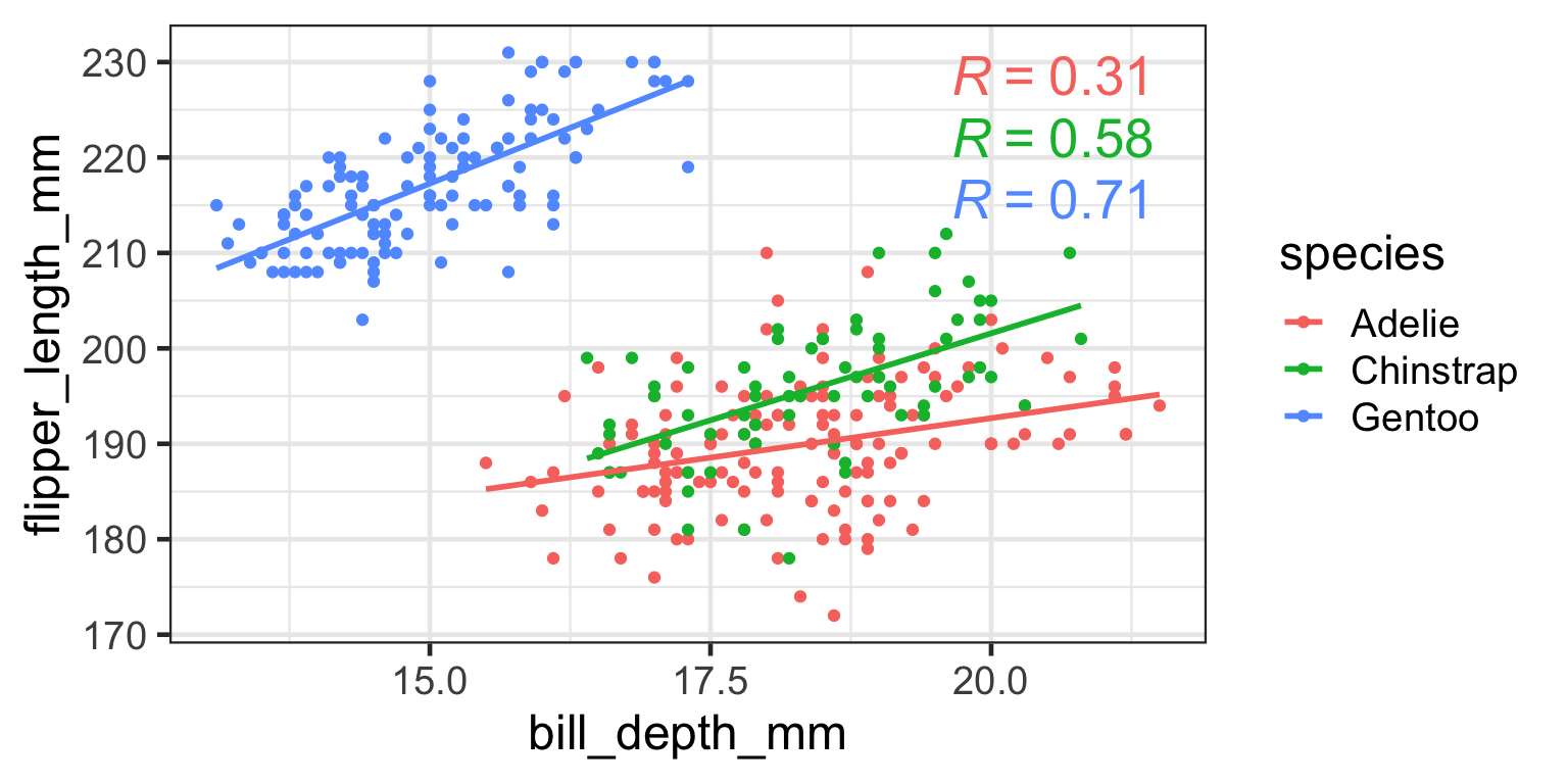
Simpson’s Paradox

• a trend appears in several groups of data but disappears or reverses when the groups are combined

Simpson’s Paradox

• a trend appears in several groups of data but disappears or reverses when the groups are combined

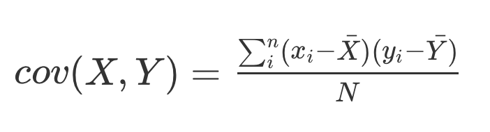
Correlation and variance

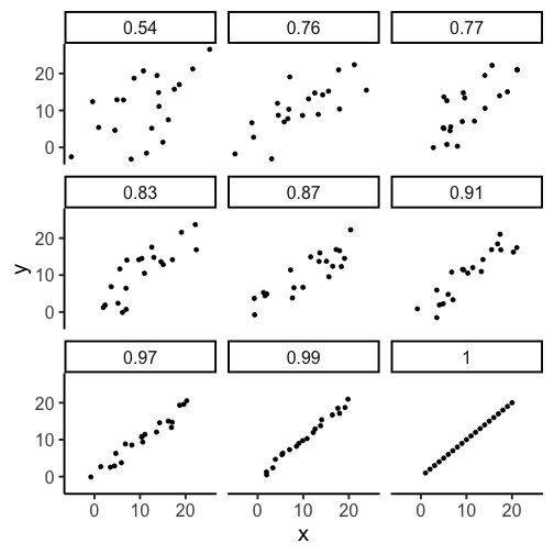
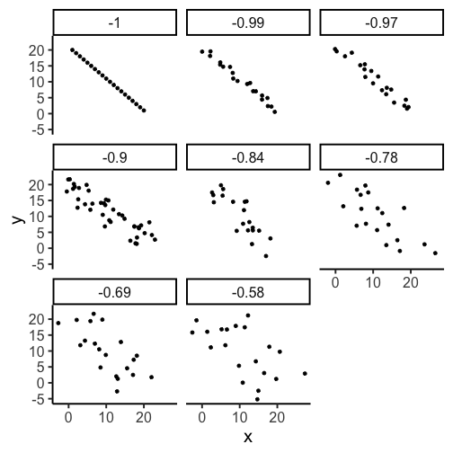
• r can be between [-1,1]
• r^2 is always between [0,1]
• r^{2} is the proportion of variance in one variable that is explained by the other variable
• r=0.5 means that 25% of the variance in one variable is explained by the other variable
• r=0.1 means that only 1% of the variance in one variable is explained by the other variable
  • (99% of the variance is unexplained by the other variable)

Correlations and Random Chance

What is randomness?

Two related ideas:

1. Things have equal chance of happening (e.g., a coin flip)

50% heads, 50% tails

Correlations and Random Chance

What is randomness?

Two related ideas:

2. Independence: One thing happening is totally unrelated to whether another thing happens

the outcome of one flip doesn’t predict the outcome of another

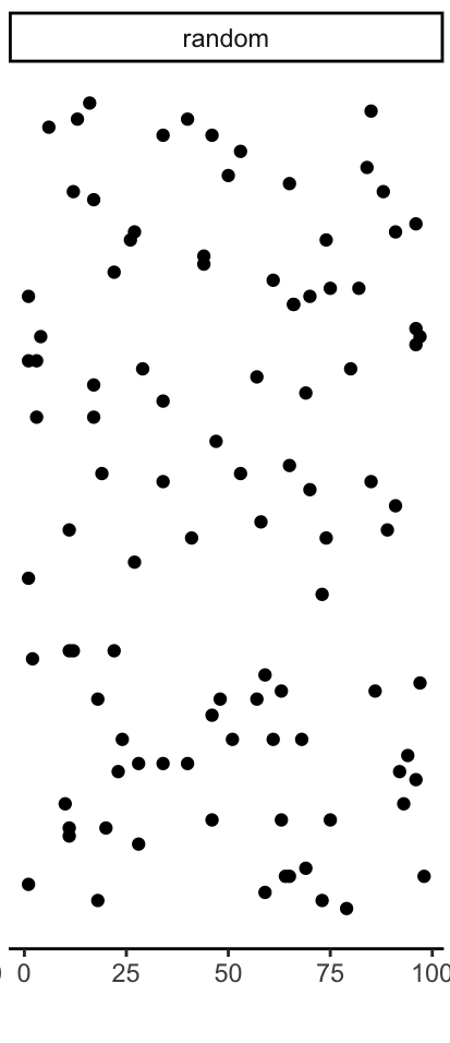
Two random variables

On average there should be zero correlation between two variables containing randomly drawn numbers

1. The numbers in variable X are drawn randomly (independently), so they do not predict numbers in Y
2. The numbers in variable Y are drawn randomly (independently), so they do not predict numbers in X

Two random variables

If X can’t predict Y, then correlation should be 0 right?

• on average yes
• for individual samples, no!

R: random numbers

In R, runif() allows you to sample random numbers (uniform distribution) between a min and max value. Numbers in the range have an equal chance of occuring

runif(n=5, min=0, max=10)

[1] 7.09529129 9.19174037 2.48744008 0.09893362 2.50790475

runif(n=5, min=0, max=10)

[1] 3.93085042 0.09306185 1.42922535 4.27942716 3.90240255

runif(n=5, min=0, max=10)

[1] 2.920361 5.632108 7.340943 3.944878 1.847596

“Random” Correlations

set.seed(28120)
x <- runif(n=5, min=0, max=10)
y <- runif(n=5, min=0, max=10)
x

[1] 2.528557 9.495890 6.832830 8.955035 5.113812

y

[1] 1.734883 7.162924 3.113391 9.979855 5.181226

cor(x,y)

[1] 0.8174196

Widget: random sampling from two random variables

What is chance capable of?

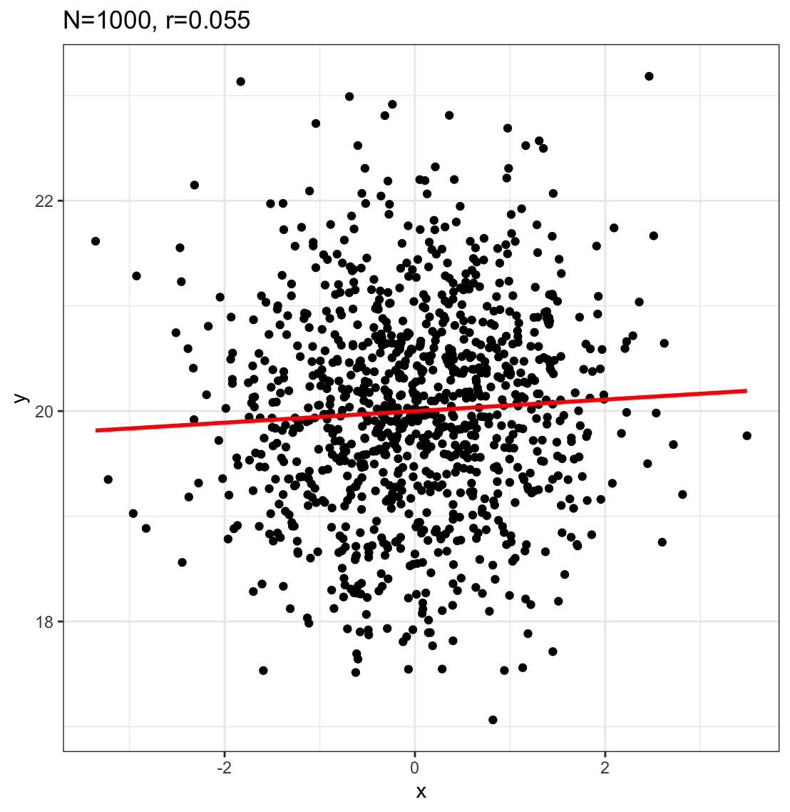
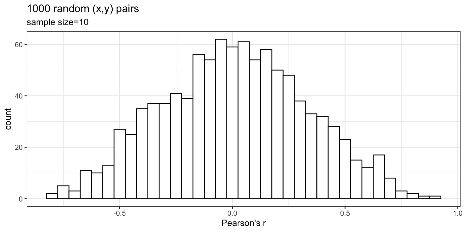
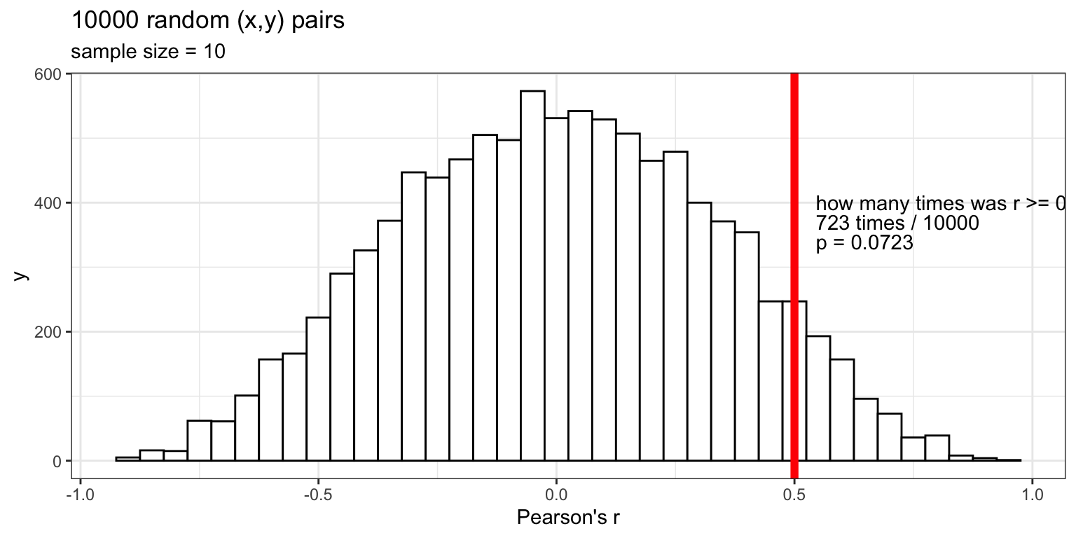
1. Randomly sampling numbers can produce a range of correlations, even when the actual correlation in the population is zero
2. What is the average correlation produced by chance? (zero)
3. For a single sample, what is the range of correlations that chance can produce?
   • answer: it depends on the sample size

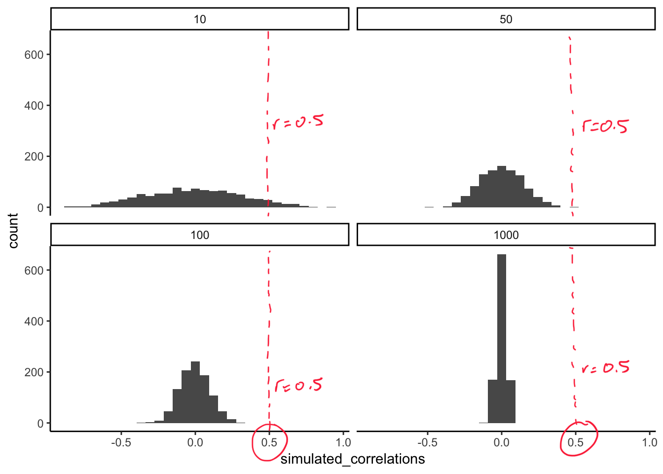
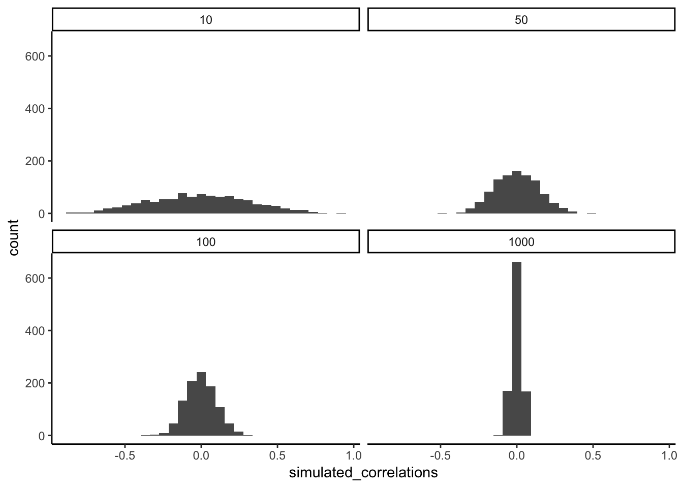
Simulating what chance can do

The role of sample size (N)

The range of chance correlations decreases as N increases

The inference problem

• Let’s say we sampled some data, and we found r = 0.5
• BUT: We know chance can sometimes produce random correlations in a sample

The inference problem

• Is the correlation we observed in our sample a reflection of a real correlation in the population?
  Is one variable really related to the other?
• Or, is there really no correlation between these variables?
• i.e. the correlation in the sample arises from random chance
  → this is H_{0}, the null hypothesis

The (simulated) Null Hypothesis

Making inferences about chance

• In a sample of size N=10, we observe: r=0.5
• Null Hypothesis H_{0}:
  → no correlation actually exists in the population
  → actual population correlation r=0.0
• Alternative Hypothesis H_{1}: correlation does exist in the population, and r=0.5 is our best estimate
• We don’t know what the truth actually is

Making inferences about chance

• We can only make an inference based on:

  What is the probability p of observing:
  → an r in a sample as big as r=0.5
  → in a sample of size N=10
  → under the null hypothesis H_{0} in which the population r=0.0

Making inferences about chance

If that probability p is low enough:
→ we conclude that it is an unlikely scenario
→ and we reject H_{0}

Making inferences about chance

How low can you go?

If that probability p is low enough:
→ we conclude that it is an unlikely scenario
→ and we reject H_{0}

How low is low enough?

• p < .05
• p < .01
• p < .001

Making inferences about chance

• cor.test() in R will give you the probability p of obtaining a sample correlation as large as you did under the null hypothesis where the population correlation is actually zero

Assumptions:
→ x vs y is a linear relationship (plot it!)
→ x & y variables are normally distributed (shapiro.test())

Making inferences about chance

ggplot(tibble(x,y), aes(x,y)) +
  geom_point(size=3) + 
  stat_poly_line(se=FALSE) +
  stat_correlation(use_label("R"), label.x="right") +
  theme_bw()

Making inferences about chance

shapiro.test(x)

    Shapiro-Wilk normality test

data:  x
W = 0.93812, p-value = 0.01136

shapiro.test(y)

    Shapiro-Wilk normality test

data:  y
W = 0.96352, p-value = 0.1248

Making inferences about chance

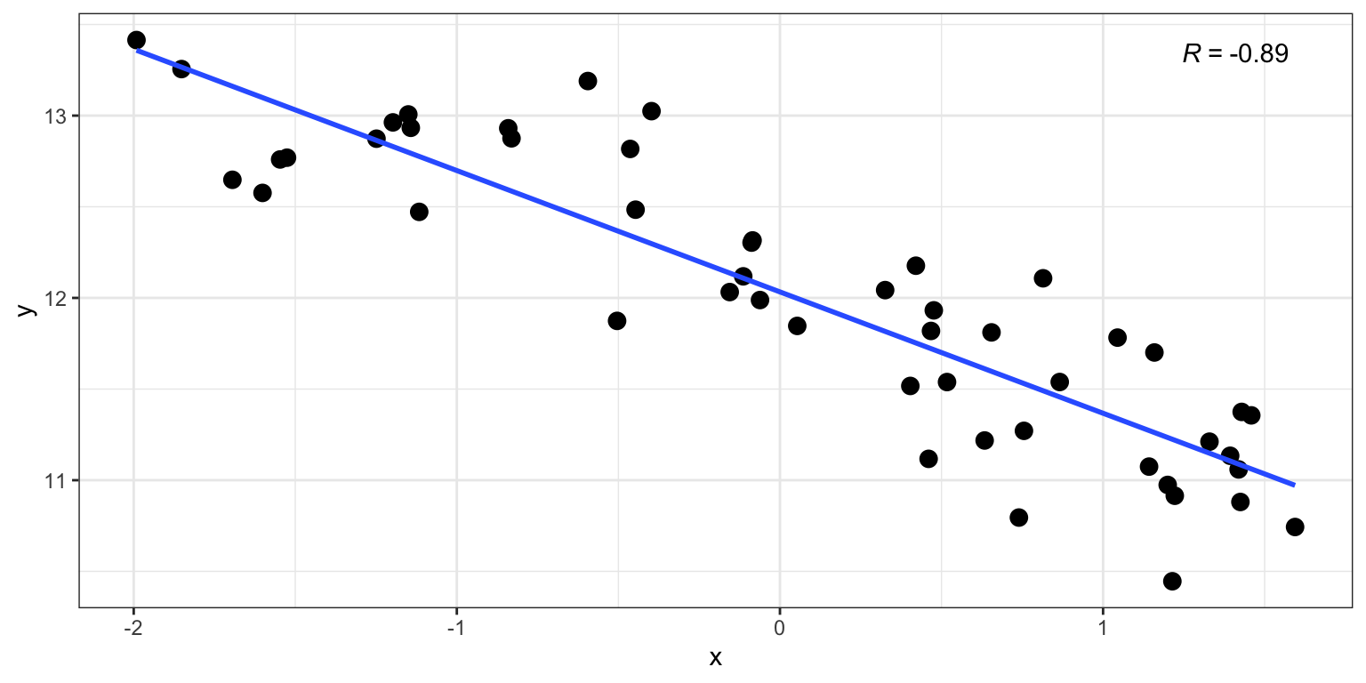
cor.test(x, y)

    Pearson's product-moment correlation

data:  x and y
t = -13.576, df = 48, p-value < 2.2e-16
alternative hypothesis: true correlation is not equal to 0
95 percent confidence interval:
 -0.9368052 -0.8142478
sample estimates:
       cor 
-0.8907193 

Making inferences about chance

• if normality assumption is not met, you can use Spearman’s rank correlation coefficient \rho (“rho”)
• See Chapter 5.7.6 of Navarro “Learning Statistics with R”

cor.test(x, y, method="spearman")

    Spearman's rank correlation rho

data:  x and y
S = 39276, p-value < 2.2e-16
alternative hypothesis: true rho is not equal to 0
sample estimates:
       rho 
-0.8860024 

IMPORTANT: “significant” \neq “large”

• significance test is not whether r is large
• test is whether r is “statistically significant”
• whether r is reliably different than 0.0

IMPORTANT: “significant” \neq “large”

• N=1000
• r=0.055
• p = 0.041
• is r significant? (yes)
• is r large? (no)
• r^{2}= .055*.055 = .003025
• = 0.3\% variance explained
  • 99.7\% of the variance is unexplained

IMPORTANT: “significant” \neq “large”

• N=7
• r=0.75
• p = 0.052
• is r significant? (no)
• is r large? (yes)