Oneway ANOVA: follow-up tests & statistical power
Week 7
Last week
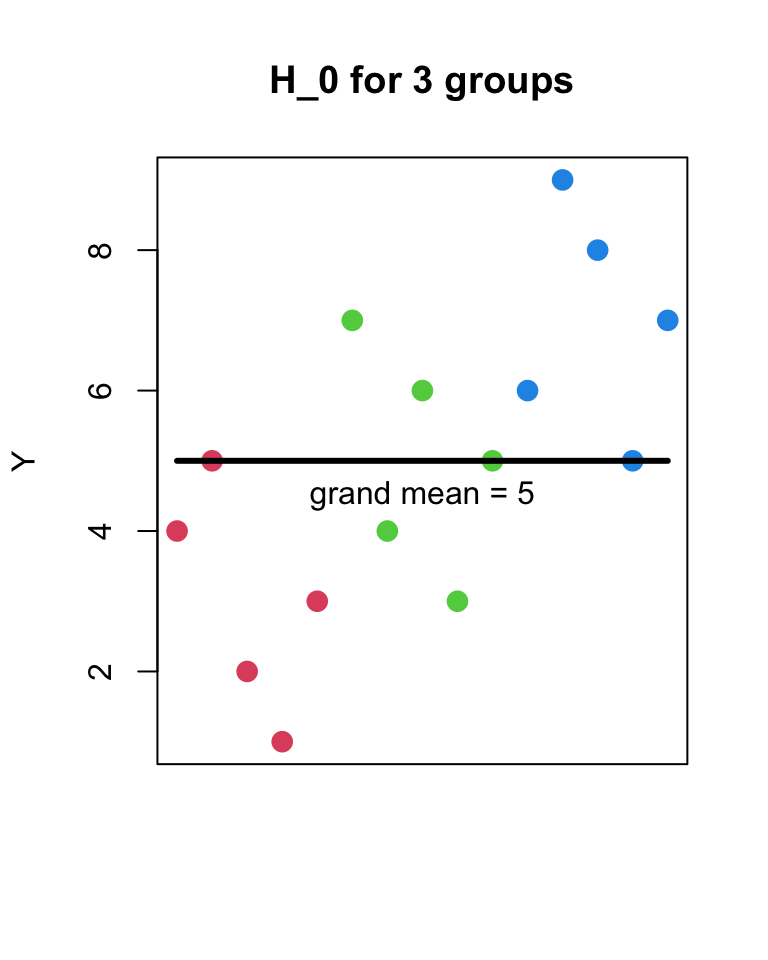
- H_{0}
- Y_{ij} = \mu + \epsilon_{ij}
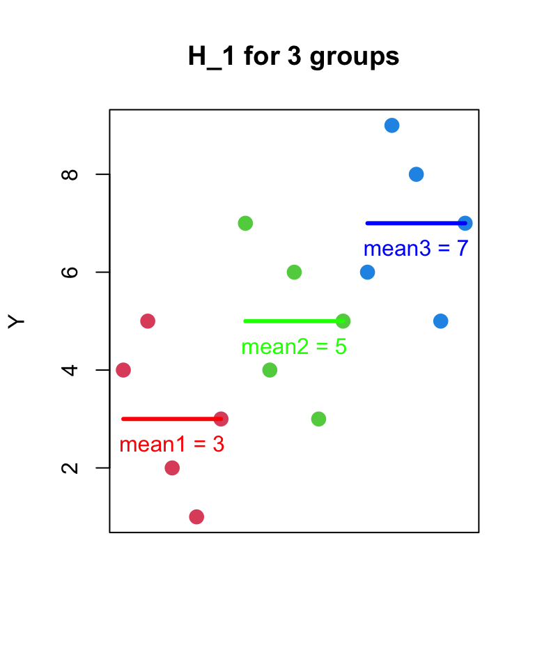
- H_{1}
- Y_{ij} = \mu_{j} + \epsilon_{ij}
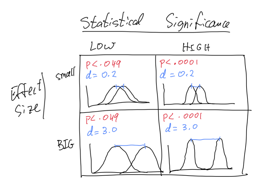
Statistical Significance vs Effect Size
- statistical significance is given by the p-value
- probability of observing a difference as large as the one we observed, under the null hypothesis H_{0} (difference between sample means due only to random sampling from same population)
- it is a metric of our confidence in the null hypothesis
Statistical Significance vs Effect Size
- effect size gives us a measure of the size of the difference between groups
- how much larger is the mean of one group compared to the mean of another group, compared to the variability within each group?
- it is a metric of the strength of the effect
Statistical Significance vs Effect Size
Effect Size: \eta^{2}
- \eta^{2} (eta-squared) is one measure of effect size
- \eta^{2} = \frac{SS_{between}}{SS_{total}}
- \eta^{2} is a proportion of the total variance that a factor explains
- ranges between 0 and 1 (just like R^{2} in regression)
- \eta^{2} is a measure of the strength of the effect
eta_quared()function in theeffectsizepackage
Effect Size: \omega^{2} & Cohen’s d
- some researchers prefer \omega^{2} (omega-squared)
- it can be less biased than \eta^{2} for small samples
- in R:
library(effectsize)andomegaSquared()function
- Cohen’s d is another measure of effect size
- it is the ratio of difference in means to the standard deviation of the groups
- in R: library(
effectsize) andcohens_d()function
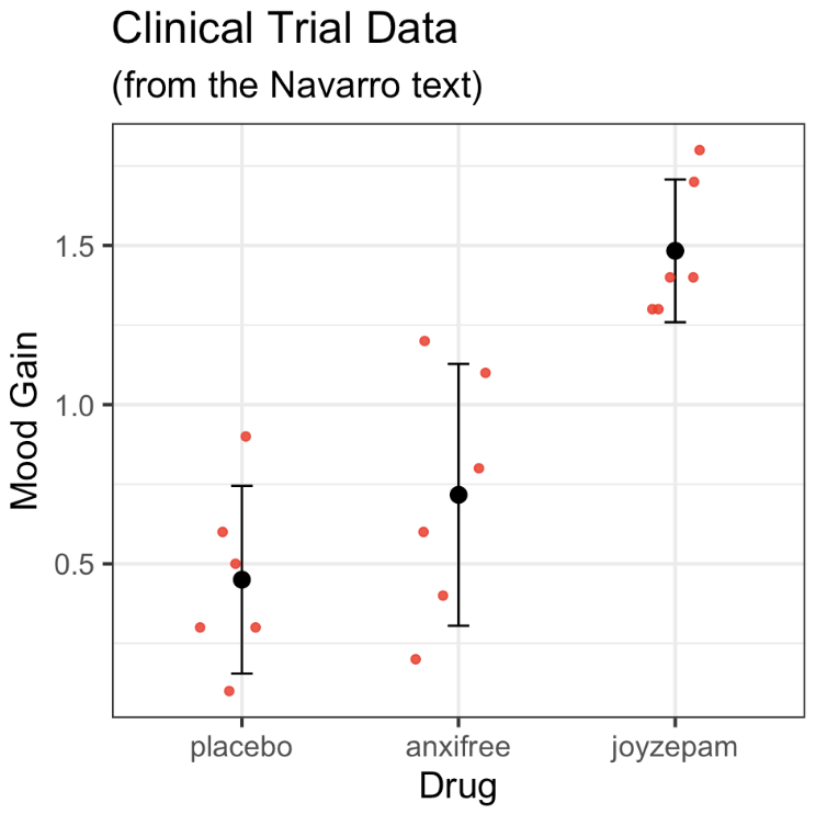
ANOVA: Omnibus F-test

- which means are different?
- we can conduct “post-hoc” tests
- like a series of pairwise t-tests
- (with some slight changes)
ANOVA: Follow-up tests


ANOVA: Follow-up tests: pairwise.t.test()
pairwise.t.test()is a function in base R- feed it your DV and your IV
pairwise.t.test( x = clin.trial$mood.gain,
                 g = clin.trial$drug,
                 p.adjust.method = "none") # we will change this later
    Pairwise comparisons using t tests with pooled SD

data:  clin.trial$mood.gain and clin.trial$drug

         placebo anxifree
anxifree 0.15021 -
joyzepam 3e-05   0.00056

P value adjustment method: none 
ANOVA: Follow-up tests: posthocPairwiseT()
posthocPairwiseT()is a function from thelsrpackage- feed it your anova model object

The Multiple Comparisons Problem
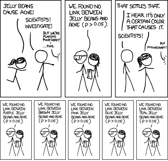
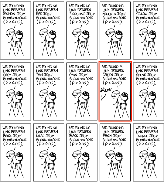
- “post-hoc” tests are like going fishing for differences
- we are testing many hypotheses on the same dataset
- Type-I errors accumulate
- actual Type-I error rate is inflated above \alpha=.05
- called “Familywise Error Rate”
- but before we get into this—let’s review Type-I and Type-II errors
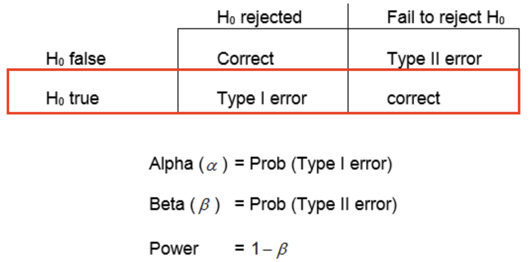
review: Type-I Errors
- a Type-I error is when you reject the null hypothesis when it is actually true
- you conclude there is a difference when there is actually no difference
review: Type-I Error rate
- how do you set the Type-I error rate?
- your threshold for rejecting the null hypothesis
- is called \alpha and is typically set to 0.05
- you are willing to make a Type-I error 5% of the time when the null hypothesis is true
Type-I Error rate: simulations
- make null hypothesis true
- take 3 samples of size 10 from one normal distribution
- all three samples come from same population (same mean)
- conduct a one-way ANOVA
- if p-value < 0.05, then reject the null hypothesis
- repeat this 10,000 times and count how many times we reject the null hypothesis
- (these are Type-I errors)
Type-I Error rate: simulations
set.seed(2812)
N <- 10                    # sample size
nsims <- 10000             # number of simulated experiments
p.values <- rep(0, nsims)   # to store our p-values
F.values <- rep(0, nsims)   # to store our F values
decisions <- rep("", nsims) # to store our decisions
for (i in seq(nsims)) {
  y1 <- rnorm(n=N, mean=0, sd=1) # sample group 1
  y2 <- rnorm(n=N, mean=0, sd=1) # sample group 2
  y3 <- rnorm(n=N, mean=0, sd=1) # sample group 3
  y <- c(y1,y2,y3)
  g <- factor(c(rep("g1",N), rep("g2",N), rep("g3",N))) # construct our group factor
  my.df <- tibble(y=y, g=g)               # construct our data tibble
  my.anova <- aov(y ~ g, data=my.df)      # conduct ANOVA
  my.anova.summary <- summary(my.anova)   # get ANOVA summary
  p <- my.anova.summary[[1]]$`Pr(>F)`[1]  # extract p-value of omnibus F-test
  F <- my.anova.summary[[1]]$`F value`[1] # extract F-value of omnibus F-test
  if (p < .05) {                          # make our decision
    decisions[i] = "reject H0"            # reject the null hypothesis
  } else {
    decisions[i] = "accept H0"            # or accept the null hypothesis
  }
  p.values[i] <- p                        # store the p-value
  F.values[i] <- F                        # store the F-value
}
my.sims <- tibble(p.values, F.values, decisions)
Type-I Error rate: simulations
# A tibble: 10,000 × 3
   p.values F.values decisions
      <dbl>    <dbl> <chr>
 1    0.668   0.409  accept H0
 2    0.878   0.130  accept H0
 3    0.950   0.0514 accept H0
 4    0.813   0.209  accept H0
 5    0.430   0.870  accept H0
 6    0.777   0.255  accept H0
 7    0.631   0.469  accept H0
 8    0.719   0.334  accept H0
 9    0.101   2.50   accept H0
10    0.827   0.191  accept H0
# ℹ 9,990 more rows
Type-I Error rate: simulations
Code
Fcrit <- sort(F.values)[round(nsims*.95)] # critical F-value
ggplot(data = my.sims, mapping = aes(x = F.values)) +
  geom_histogram(bins = 100,
                 fill = "transparent",
                 color = "black") +
  geom_vline(xintercept = Fcrit, color = "red", size = 1) +
  theme_bw() + labs(title = "F values under H0",
                      subtitle = sprintf("n=%d simulated experiments", nsims))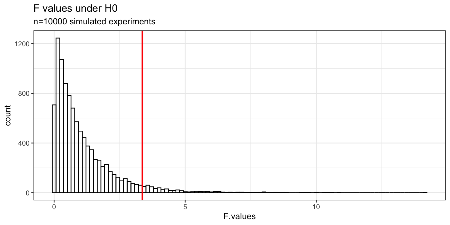
Type-I Error rate: simulations
Code
my.sims <- tibble(p.values, F.values, decisions)
ggplot(data = my.sims, mapping = aes(x = p.values)) +
  geom_histogram(breaks = seq(0,1,0.01),
                 fill = "transparent",
                 color = "black") +
  geom_vline(xintercept = .05, color = "red", size = 1) +
  theme_bw() + labs(title = "p-values under H0",
                    subtitle = sprintf("n=%d simulated experiments", nsims))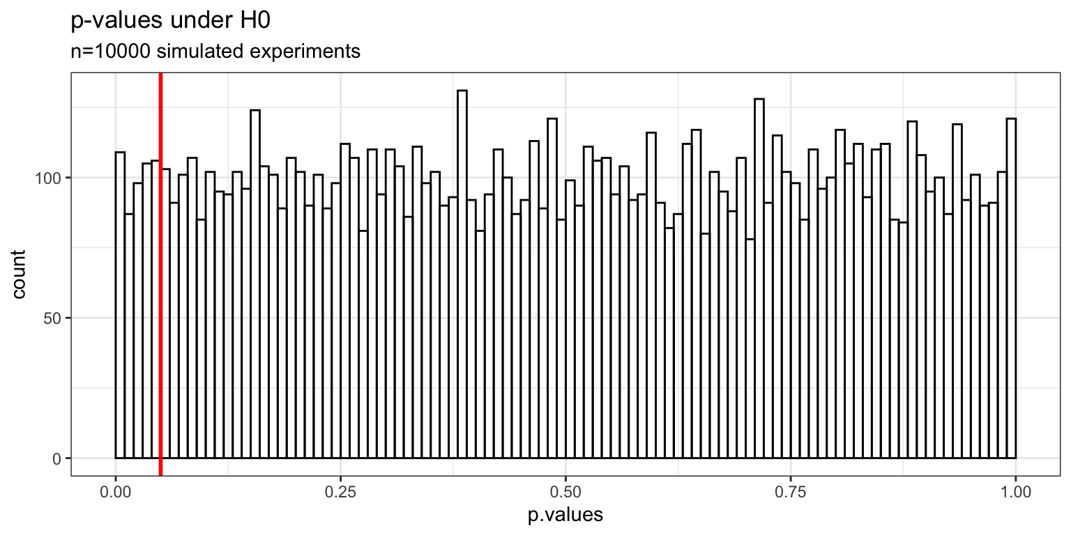
Type-I Error rate: simulations
# A tibble: 2 × 3
  decisions     n percent
  <chr>     <int>   <dbl>
1 accept H0  9495  0.950
2 reject H0 505 0.0505- decision based on \alpha=.05, so we made 5% Type-I errors
- if decision based on \alpha=.01, we make 1% Type-I errors
- if decision based on \alpha=.001, we make 0.1% Type-I errors
- you get to choose your Type-I error rate
Type-I Error rate
- important: we never know whether H_{0} is true or H_{1} is true
- we compute p under the assumption that H_{0} is true
- decision to reject or accept H_{0} based on comparing p to \alpha
Type-I Error rate
- H_{0} is actually true: then \alpha determines our Type-I error rate
- H_{0} is actually false: rejecting H_{0} is the correct decision; no Type-I error

Type-II Error rate
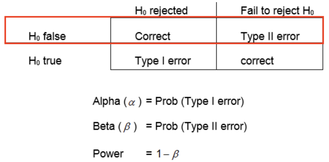
- a Type-II error is when you fail to reject the null hypothesis even though it is actually false—the alternate hypothesis is true
- you conclude there is not a difference when there is actually is one
Type-II Error rate
- \beta is the probability of making a Type-II error
- the power of your statistical test is defined as 1-\beta
- statistical power is the probability of correctly rejecting the null hypothesis when it is false
- the probability that you will correctly detect a difference when there is one
Determinants of statistical power
- effect size
- how big is the difference between the groups relative to within-group variance?
- sample size
- bigger sample size: more power to detect a difference when there is one
- \alpha
- smaller \alpha: less power to detect a difference when there is one
Computing power in R
power.anova.test()will compute power for an ANOVApower.t.test()will compute power for a t-test- important: power calculations are always based on the assumption that H_{1} is true
- (groups came from different populations with different means)
Power example: ANOVA (H_{1} true)
- we have 3 groups; we want to detect a difference between groups with a power of 0.8
- assume H_{1} is true: we expect within-groups variance to be 4 times as big as the between-groups variance
     Balanced one-way analysis of variance power calculation

         groups = 3
              n = 20.30205
    between.var = 1
     within.var = 4
      sig.level = 0.05
          power = 0.8

NOTE: n is number in each grouppower.anova.test()tells us we would need n=20 subjects per group to detect a difference between groups with a power of 0.8
Power example: ANOVA (H_{1} true)
     Balanced one-way analysis of variance power calculation

         groups = 3
              n = 20.30205
    between.var = 1
     within.var = 4
      sig.level = 0.05
          power = 0.8

NOTE: n is number in each group- if there actually is a difference in the population and we run this experiment 100 times, 80 times out of 100 we will correctly reject the null hypothesis
- 20 times out of 100 we will make a Type-II error and conclude there is not a difference
- play with parameters to see how sample size n depends on power and effect size
Power example: ANOVA (H_{0} true)
- if there actually is NOT a difference in the population:
- and if we adopt \alpha=0.05:
- if we run this experiment 100 times, 95 times out of 100 we will correctly fail to reject the null hypothesis
- 5 times out of 100 we will make a Type-I error and conclude there is a difference even though there isn’t
- this is because our decision to reject or fail to reject H_{0} is based on comparing p to \alpha=0.05
Multiple Comparisons
- how many possible pairwise tests?
- placebo vs anxifree
- placebo vs joyzepam
- anxifree vs joyzepam
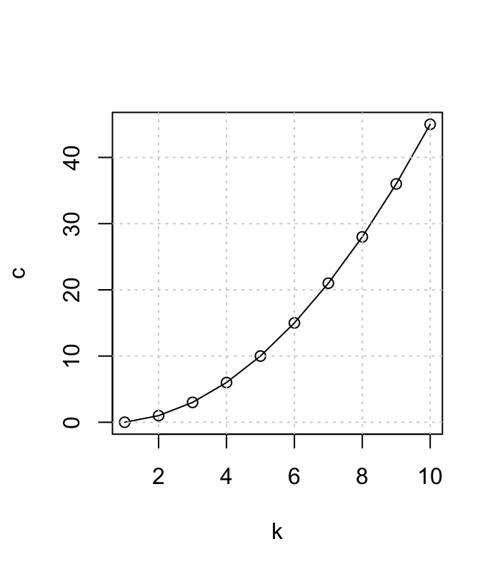
- For K groups the number of possible pairwise comparisons c is:
- c = K(K-1)/2

Multiple Comparisons
- For K groups the number of possible pairwise comaprisons c is:
- c = K(K-1)/2
- for 3 groups: 3*(3-1)/2 = 3
- for 4 groups: 4*(4-1)/2 = 6
- for 6 groups: 6*(6-1)/2 = 15
- for 10 groups: 10*(10-1)/2 = 45 !
Multiple Comparisons
- 3 post-hoc tests:
- placebo vs anxifree
- placebo vs joyzepam
- anxifree vs joyzepam
- each test has a p-value
- we make a decision about each test based on \alpha = .05
- Q: is our overal (family-wise) Type-I error rate still 5 %?

Multiple Comparisons
- is family-wise Type-I error still 5 %?
- Answer: No!
- Type-I error rate is inflated
- Type-I error rate on the whole family of tests is way above 5 %
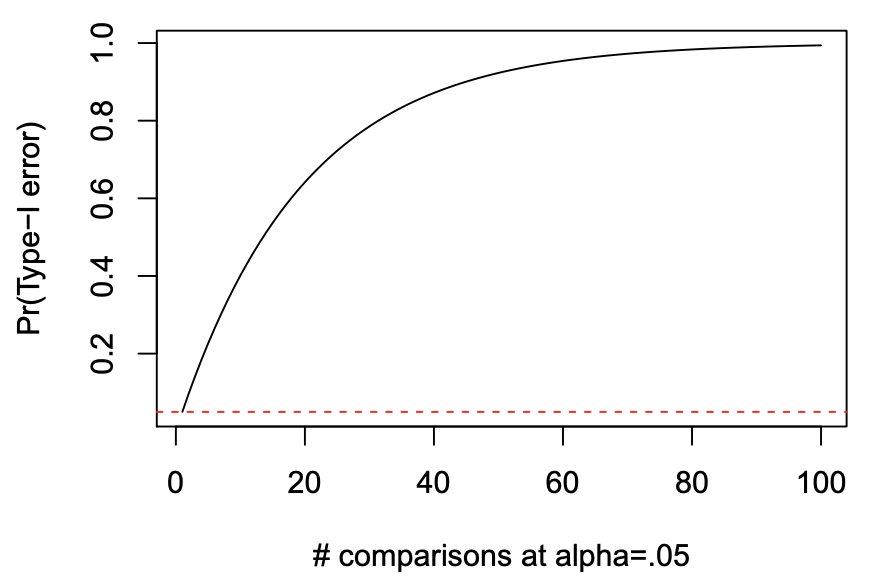
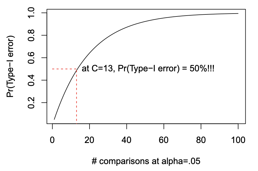
- Pr(Type-I error) = 1 - (1 - \alpha)^{C}
- C is the number of post-hoc tests

Multiple Comparisons
- Pr(Type-I error) = 1 - (1 - \alpha)^{C}
- when C=3
- we get 14.3% family-wise Type-I error rate

Multiple Comparisons
- Pr(Type-I error) = 1 - (1 - \alpha)^{C}
Multiple Comparisons
- Pr(Type-I error) = 1 - (1 - \alpha)^{C}
Why does Type-I error rate inflate?
- when we do post-hoc tests, we are increasing the number of tests performed on the same dataset
- the more tests we do, the more likely to make a Type-I error
- especially if we look at the data first and test the differences that look largest
- we end up chasing the big differences
- big differences (even if they are due to chance) are more likely to be identified as statistically significant
Correcting for Type-I error inflation
- there are several ways to correct for Type-I error inflation
- we will look at three of them:
- Bonferroni
- Tukey
- Bonferroni-Holm
Bonferroni Correction
- corrects for Type-I error inflation
- p_{\mathrm{corrected}} becomes p * C for each test
- if C=3 then p_{\mathrm{corrected}}=0.05*3=0.15
- for each test, reject H_{0} only if p_{\mathrm{corrected}}<0.05
- simple, but overly conservative when doing many tests
Bonferroni Correction in R
Tukey Correction
- allows for all pairwise comparisons among groups even when there are many
- still maintains overall \alpha = 0.05
- less conservative than Bonferroni when doing a large number of tests
- corrects the p-value with a formula based on number of groups
- reject H_{0} when p_{\mathrm{corrected}}<0.05
Tukey Correction in R
  Tukey multiple comparisons of means
    95% family-wise confidence level

Fit: aov(formula = mood.gain ~ drug, data = clin.trial)

$drug
                       diff        lwr       upr     p adj
anxifree-placebo  0.2666667 -0.1901184 0.7234518 0.3115006
joyzepam-placebo  1.0333333  0.5765482 1.4901184 0.0000854
joyzepam-anxifree 0.7666667  0.3098816 1.2234518 0.0015284
Bonferroni-Holm Correction
- a good general purpose correction
- less conservative than Bonferroni & Tukey
- still allows for any number of pairwise comparisons
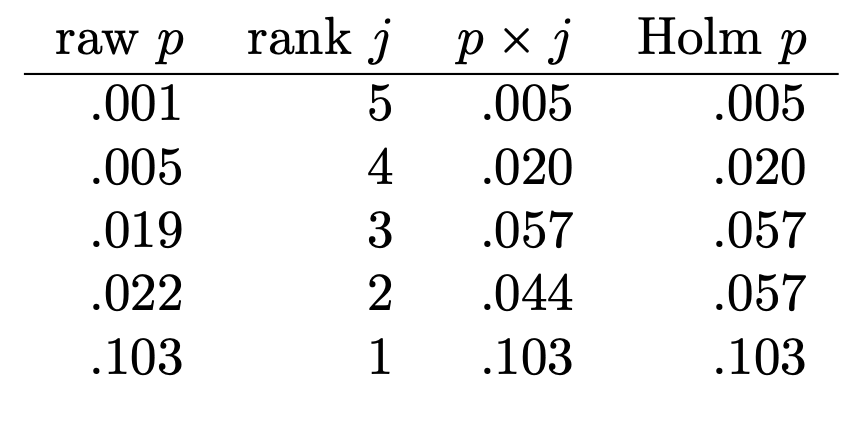
- sorts tests by uncorrected p-value
- then corrects p-values more for most significant tests and less for less significant tests
- reject H_{0} when p_{\mathrm{corrected}}<0.05
Bonferroni-Holm Correction
- corrects more for most significant tests and less for less significant tests
Bonferroni-Holm Correction in R
Unbalanced Designs
- when we have unequal sample sizes in the ANOVA groups
- can be a problem for the ANOVA test
- think about why? (e.g. homogeneity of variances)
- calculations to correct for unequal sample sizes are complicated and tedious
- sometimes reasonable people even disagree on the best approach
- try hard not to have unequal sample sizes in your ANOVA groups!!
- we will return to this later in the course when we talk about Factorial ANOVA
- as we saw in a previous lecture, for oneway ANOVA you can use Welch’s
oneway.test()if you are concerned about homogeneity of variance due to unequal sample sizes
(see Navarro, Ch. 14.8 for details)
