Oneway ANOVA & the GLM

Week 6

T-test

two samples
are they from two populations with different means?
or are they from one or more populations with the same mean?
- (and sample differences are due to random chance?)

# A tibble: 12 × 2
       x g        
   <dbl> <fct>    
 1    67 control  
 2   103 control  
 3   109 control  
 4    74 control  
 5    93 control  
 6   106 control  
 7   115 treatment
 8   124 treatment
 9   130 treatment
10   120 treatment
11   138 treatment
12   126 treatment

          g     x
1   control  92.0
2 treatment 125.5

T-test

what is the probability of taking two samples of size N=6 from population(s) with the same mean and observing a difference in means as large as the one observed?
this is the probability of observing the data under H_{0}, the null hypothesis

# A tibble: 12 × 2
       x g        
   <dbl> <fct>    
 1    67 control  
 2   103 control  
 3   109 control  
 4    74 control  
 5    93 control  
 6   106 control  
 7   115 treatment
 8   124 treatment
 9   130 treatment
10   120 treatment
11   138 treatment
12   126 treatment

          g     x
1   control  92.0
2 treatment 125.5

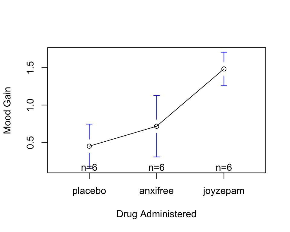
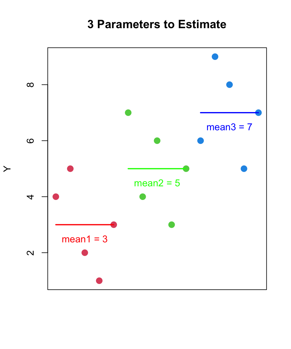
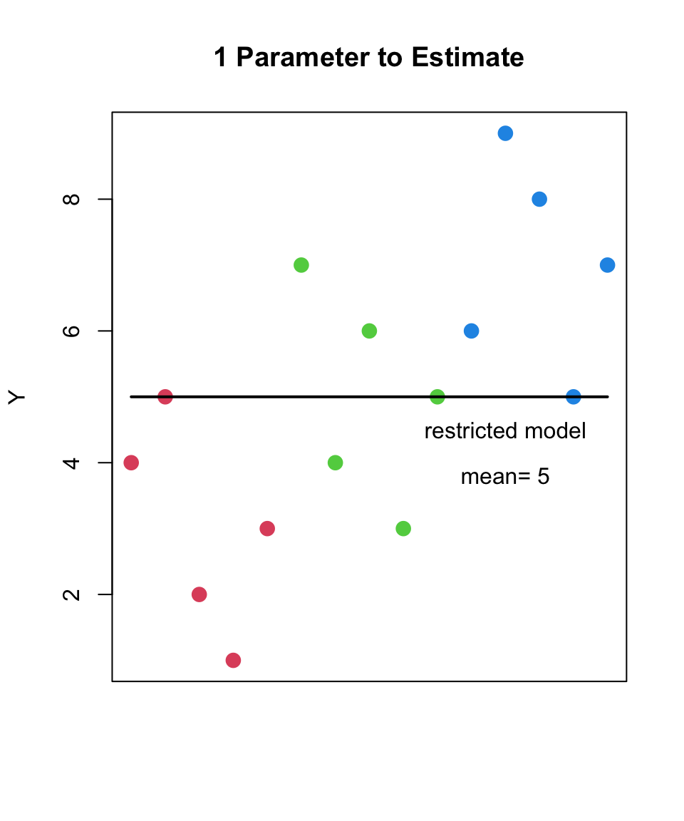
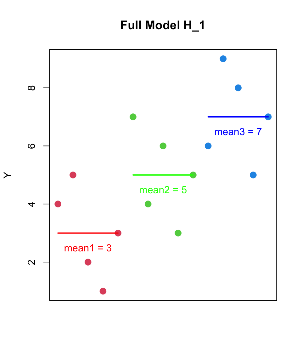
ANOVA: N groups

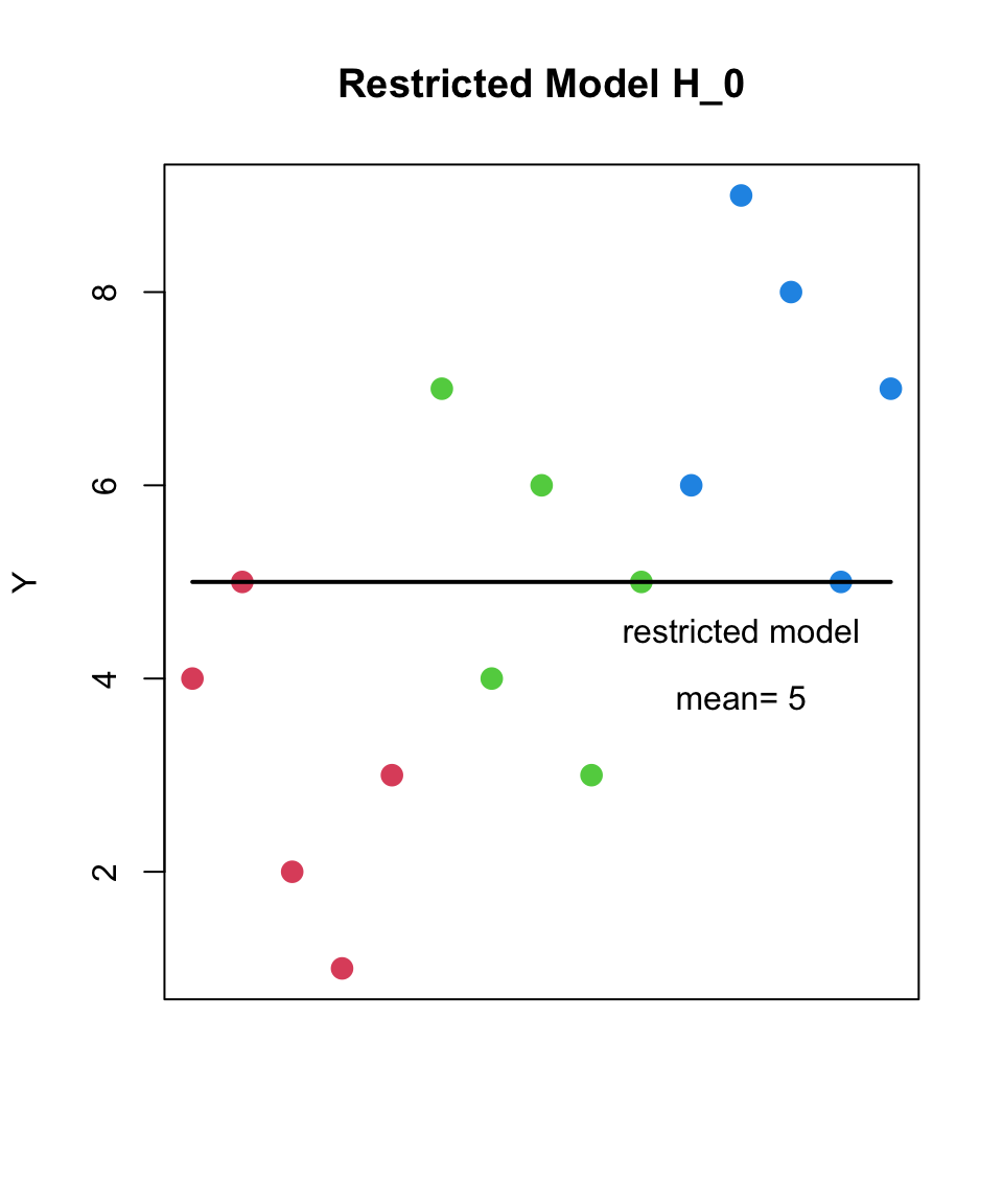
H_{0}: groups sampled from population(s) with the same mean
H_{1}: groups not sampled from populations(s) with the same mean
- (i.e. at least one group was sampled from a population with a different mean)
p-value: what is the probability of observing differences between groups as large as the ones observed, if H_{0} is true?
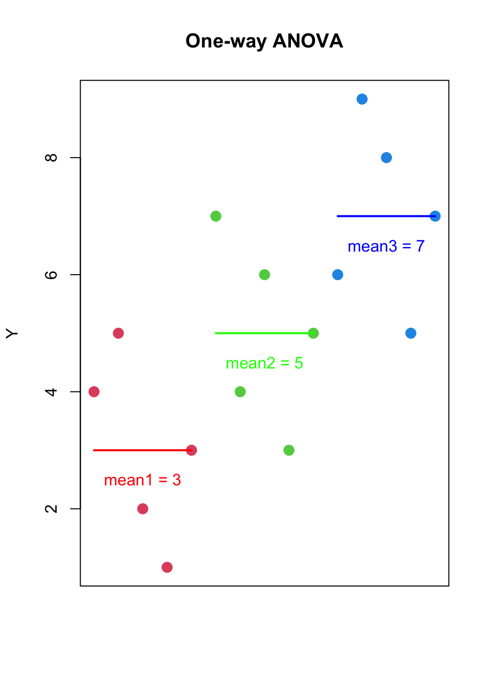
- if we sampled three groups of size N=4 from population(s) with the same mean?

# A tibble: 12 × 2
       x g         
   <dbl> <fct>     
 1    86 treatment1
 2    89 treatment1
 3   109 treatment1
 4   110 treatment1
 5   124 treatment2
 6   105 treatment2
 7    90 treatment2
 8   112 treatment2
 9   127 treatment3
10   121 treatment3
11   110 treatment3
12   134 treatment3

           g      x
1 treatment1  98.50
2 treatment2 107.75
3 treatment3 123.00

ANOVA

ANOVA stands for ANalysis Of VAriance
ANOVA is a statistical test that compares the means of two or more groups
many forms of ANOVA exist, but we will start with the simplest:
- one-way between-subjects ANOVA
(read Navarro, chapter 14)

one-way between-subjects ANOVA

one-way: one independent variable
- later we will see two-factor ANOVA and n-factor ANOVA
between-subjects: each participant contributes an observation in only one group
- later we will see within-subjects ANOVA and mixed ANOVA

Omnibus F-test

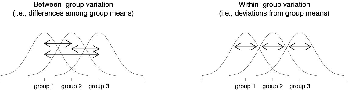
ANOVA computes an “omnibus” F-statistic, which is a ratio of two variances
- (omnibus means “overall”)
- the numerator is the between-groups variance
- the denominator is the within-groups variance
Omnibus F-statistic is a metric of the “overall” question:
- “are the means of the groups the same? (or not the same)?”

Omnibus F-test

Omnibus F-test

F = \frac{\mathrm{BetweenVariance}}{\mathrm{WithinVariance}}
what is F going to be?
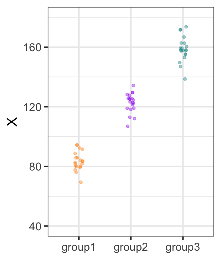
F-ratio far above 1.0: between-groups variance is larger than within-groups variance

Omnibus F-test

F = \frac{\mathrm{BetweenVariance}}{\mathrm{WithinVariance}}
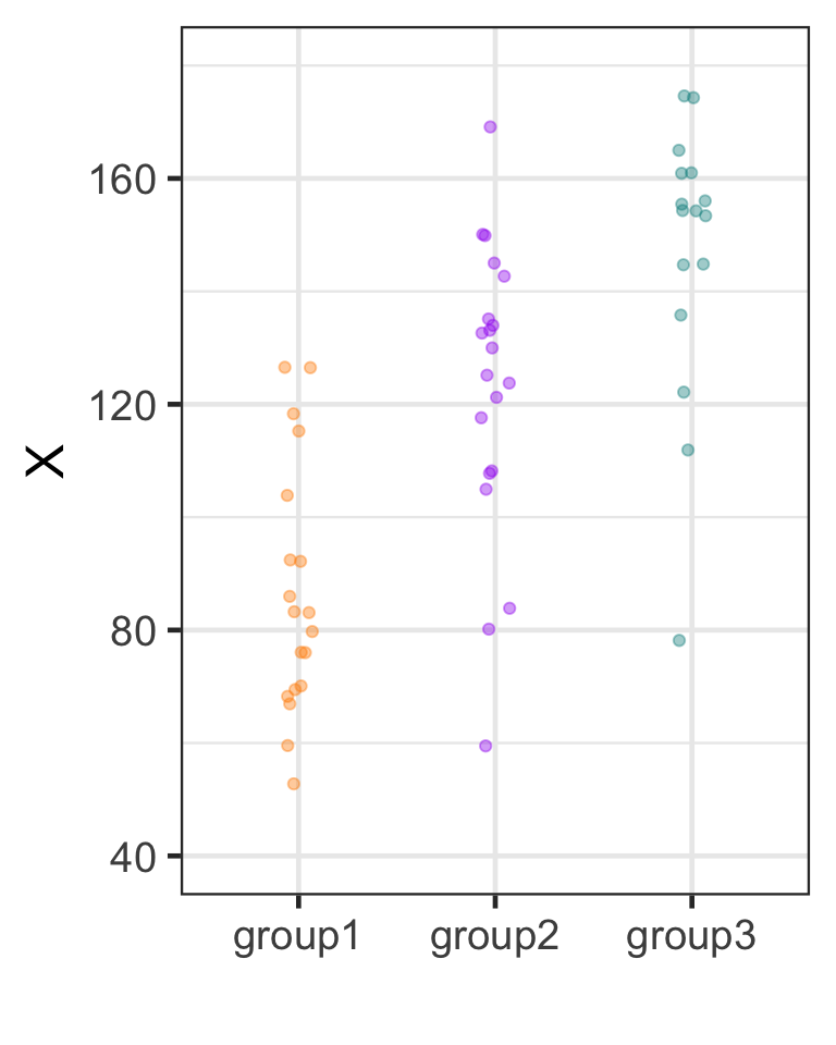
what is F going to be?
F-ratio below 1.0: between-groups variance is smaller than within-groups variance

Omnibus F-test

null hypothesis is that the population means of all groups are equal
- H_{0}: each group was sampled from population(s) with the same mean
- H_{1}: at least one group was sampled from a population with a different mean
the p-value for the omnibus F-test is the probability of observing an F-statistic as large as the one computed, assuming that the null hypothesis is true

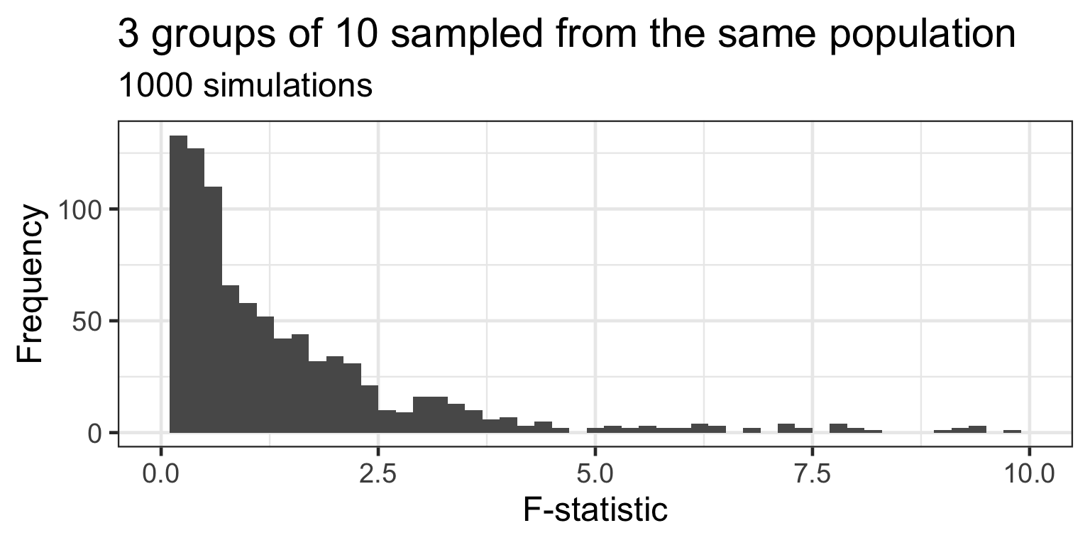
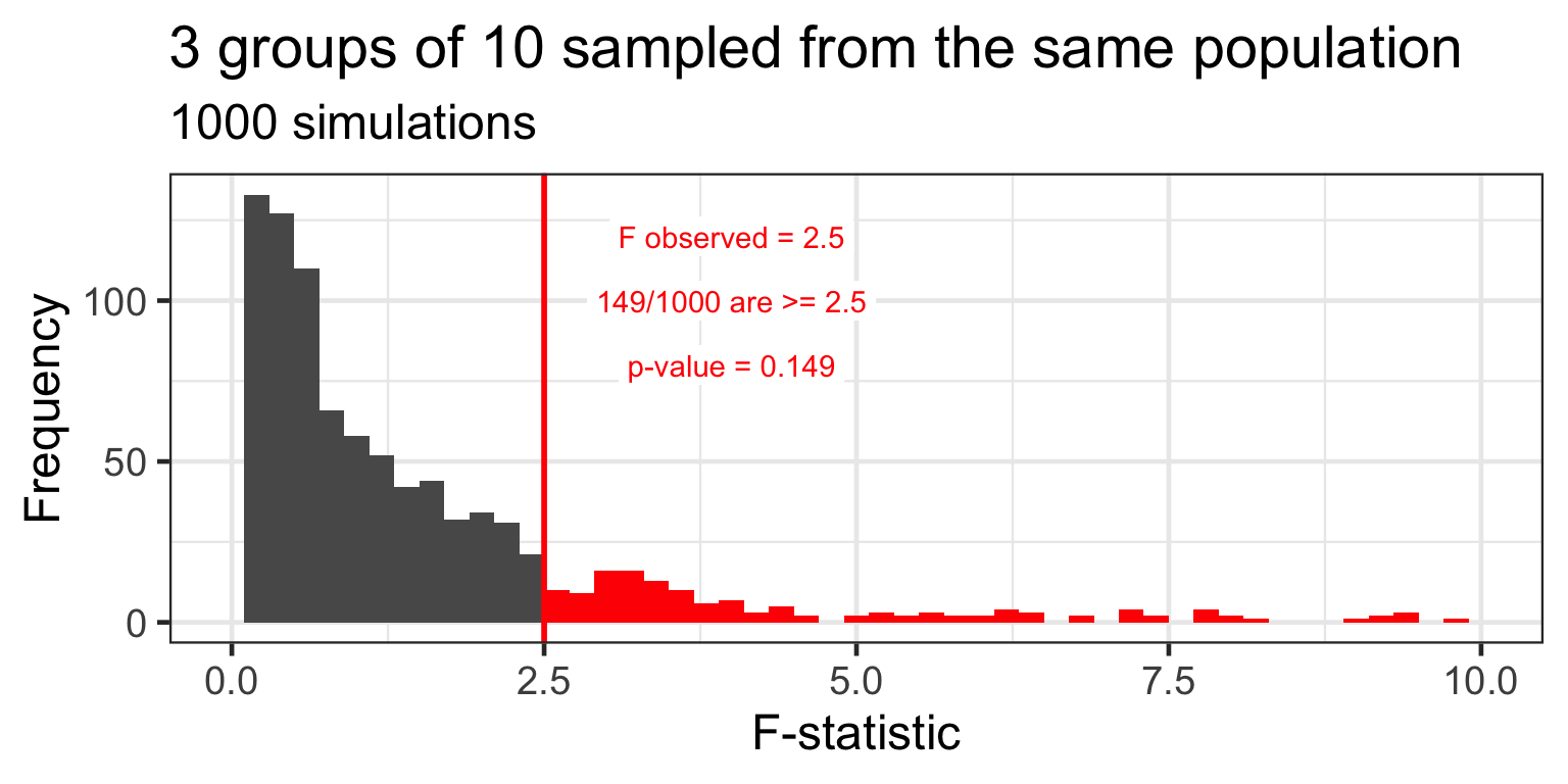
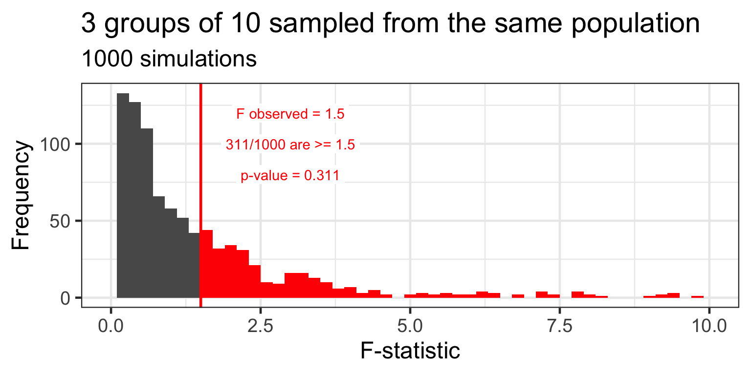
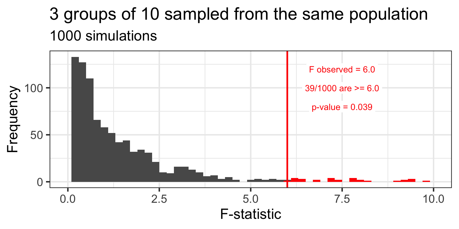
Distribution of F under H_{0}

under the null hypothesis, groups are sampled from population(s) with the same mean
but random sampling results in differences between sample groups
the F-statistic is an overall (omnibus) measure of the differences between all groups
under the null hypothesis we expect the F-statistic to be close to 1.0 most of the time
but due to random sampling, under the null hypothesis, sometimes it will be larger
the p-value tells us how likely is it to observe a given F-statistic under H_{0}

Distribution of F under H_{0}

Omnibus F-test

following a significant omnibus F-test, we can perform follow-up tests to determine which groups differ from each other
not this week—we will cover follow-up tests next week
If the omnibus F-test is not significant, we should stop
- Omnibus F-test protects us from making more Type I errors than we want
- more about this next week

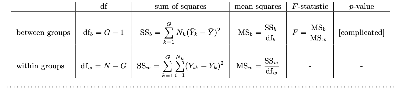
ANOVA Table/Formulas

\mathrm{SS_{b}} = sum of squares between
- each group mean minus the grand mean of all groups
\mathrm{SS_{w}} = sum of squares within
- each observation minus the group mean to which it belongs

ANOVA Table/Formulas

read Navarro, chapter 14, for a worked example, going from the raw data to the ANOVA table
today, we will use R to compute the ANOVA table

An illustrative dataset

sample data file from Navarro text: clinicaltrial.Rdata

library(tidyverse)
load(url("https://www.gribblelab.org/2812/data/clinicaltrial.Rdata"))

(clin.trial <- tibble(clin.trial))

# A tibble: 18 × 3
   drug     therapy    mood.gain
   <fct>    <fct>          <dbl>
 1 placebo  no.therapy       0.5
 2 placebo  no.therapy       0.3
 3 placebo  no.therapy       0.1
 4 anxifree no.therapy       0.6
 5 anxifree no.therapy       0.4
 6 anxifree no.therapy       0.2
 7 joyzepam no.therapy       1.4
 8 joyzepam no.therapy       1.7
 9 joyzepam no.therapy       1.3
10 placebo  CBT              0.6
11 placebo  CBT              0.9
12 placebo  CBT              0.3
13 anxifree CBT              1.1
14 anxifree CBT              0.8
15 anxifree CBT              1.2
16 joyzepam CBT              1.8
17 joyzepam CBT              1.3
18 joyzepam CBT              1.4

DV is mood.gain
IV is drug
drug is a factor with 3 levels
- placebo (n=6)
- anxifree (n=6)
- joyzepam (n=6)
any factors in your dataset must be set in R as a factor <fct> — this is critical for computing ANOVA in R
- factor() will convert numbers or characters to a <fct>
for now let’s ignore the therapy factor in the dataset.

An illustrative dataset

Code

clin.trial <- clin.trial %>%
    select(-therapy)
clin.trial

# A tibble: 18 × 2
   drug     mood.gain
   <fct>        <dbl>
 1 placebo        0.5
 2 placebo        0.3
 3 placebo        0.1
 4 anxifree       0.6
 5 anxifree       0.4
 6 anxifree       0.2
 7 joyzepam       1.4
 8 joyzepam       1.7
 9 joyzepam       1.3
10 placebo        0.6
11 placebo        0.9
12 placebo        0.3
13 anxifree       1.1
14 anxifree       0.8
15 anxifree       1.2
16 joyzepam       1.8
17 joyzepam       1.3
18 joyzepam       1.4

how many participants in each group?

xtabs( ~drug, clin.trial )

drug
 placebo anxifree joyzepam 
       6        6        6

mean of each group?

aggregate( mood.gain ~ drug, clin.trial, mean )

      drug mood.gain
1  placebo 0.4500000
2 anxifree 0.7166667
3 joyzepam 1.4833333

sd of each group?

aggregate( mood.gain ~ drug, clin.trial, sd )

      drug mood.gain
1  placebo 0.2810694
2 anxifree 0.3920034
3 joyzepam 0.2136976

An illustrative dataset

# A tibble: 18 × 2
   drug     mood.gain
   <fct>        <dbl>
 1 placebo        0.5
 2 placebo        0.3
 3 placebo        0.1
 4 anxifree       0.6
 5 anxifree       0.4
 6 anxifree       0.2
 7 joyzepam       1.4
 8 joyzepam       1.7
 9 joyzepam       1.3
10 placebo        0.6
11 placebo        0.9
12 placebo        0.3
13 anxifree       1.1
14 anxifree       0.8
15 anxifree       1.2
16 joyzepam       1.8
17 joyzepam       1.3
18 joyzepam       1.4

or, using our dplyr/tidyverse skills:

clin.trial %>% 
    group_by(drug) %>% 
    summarise(n = n(),
              mean = mean(mood.gain),
              sd = sd(mood.gain))

# A tibble: 3 × 4
  drug         n  mean    sd
  <fct>    <int> <dbl> <dbl>
1 placebo      6 0.45  0.281
2 anxifree     6 0.717 0.392
3 joyzepam     6 1.48  0.214

An illustrative dataset

# A tibble: 18 × 2
   drug     mood.gain
   <fct>        <dbl>
 1 placebo        0.5
 2 placebo        0.3
 3 placebo        0.1
 4 anxifree       0.6
 5 anxifree       0.4
 6 anxifree       0.2
 7 joyzepam       1.4
 8 joyzepam       1.7
 9 joyzepam       1.3
10 placebo        0.6
11 placebo        0.9
12 placebo        0.3
13 anxifree       1.1
14 anxifree       0.8
15 anxifree       1.2
16 joyzepam       1.8
17 joyzepam       1.3
18 joyzepam       1.4

plotmeans() from the gplots package

library(gplots)
plotmeans( formula = mood.gain ~ drug,
  data = clin.trial,
  xlab = "Drug Administered",
  ylab = "Mood Gain"
 )

An illustrative dataset

or the ggplot way:

clin.trial %>% 
    group_by(drug) %>% 
    summarise(mood = mean(mood.gain),
              sd   = sd(mood.gain),
              N    = n(),
              se   = sd/sqrt(N),
              ci95 = se * qt(.975,N-1)) %>%
    ggplot(aes(x=drug,y=mood)) +
        geom_errorbar(aes(ymin  = mood-ci95, 
                          ymax  = mood+ci95),
                          width = 0.1) +
        geom_point(aes(x=drug,y=mood),
                   size = 3) + 
        geom_jitter(data=clin.trial, 
                    aes(x=drug,y=mood.gain),
                    width = 0.1,
                    color = "red",
                    alpha = 0.8) + 
        labs(x="Drug", y="Mood Gain",
             title="Clinical Trial Data",
             subtitle="(from the Navarro text)") + 
        theme_bw(base_size=16)

The ANOVA Omnibus F-test

Are differences between group means real^{*} or due to random chance?
what is the probability of observing differences as big as this if the null hypothesis is true?
H_{0}: each group was sampled from population(s) with the same mean
H_{1}: it is not true that each group was sampled from population(s) with the same mean

The ANOVA Omnibus F-test

Are differences between group means real^{*} or due to random chance?
what is the probability of observing differences as big as this if the null hypothesis is true?
Omnibus F-test: F = \frac{\mathrm{MS_{between}}}{\mathrm{MS_{within}}}
- gives an overall measure of the difference between all group means together, relative to the variability within each group

ANOVA in R - `aov()`

my.anova <- aov( mood.gain ~ drug, data = clin.trial )
summary(my.anova)

            Df Sum Sq Mean Sq F value   Pr(>F)    
drug         2  3.453  1.7267   18.61 8.65e-05 ***
Residuals   15  1.392  0.0928                     
---
Signif. codes:  0 '***' 0.001 '**' 0.01 '*' 0.05 '.' 0.1 ' ' 1

ANOVA in R - `aov()`

my.anova <- aov( mood.gain ~ drug, data = clin.trial )
summary(my.anova)

            Df Sum Sq Mean Sq F value   Pr(>F)    
drug         2  3.453  1.7267   18.61 8.65e-05 ***
Residuals   15  1.392  0.0928                     
---
Signif. codes:  0 '***' 0.001 '**' 0.01 '*' 0.05 '.' 0.1 ' ' 1

p < 0.05, so we reject the null hypothesis
The groups were not sampled from population(s) with the same mean
What is differerent from what??
We don’t know yet, the omnibus F-test just tells us that there are differences somewhere

ANOVA in R : follow-up tests

next week we will talk about post-hoc tests, which allow us to determine which groups are different from each other
an issue of great importance is Type-I Error rate
more on this next week

ANOVA Assumptions

Normality of the residuals
Homogeneity of variance across groups
Independence of observations

1. Normality

residuals are assumed to be normally distributed
plot a histogram of the residuals
plot a Q-Q plot (quantile-quantile plot)
Shapiro-Wilk hypothesis test

1. Normality

hist(residuals(my.anova))

qqnorm(y=residuals(my.anova),pch=16)
qqline(y=residuals(my.anova),lty=2)

1. Normality

shapiro.test(residuals(my.anova))


    Shapiro-Wilk normality test

data:  residuals(my.anova)
W = 0.96019, p-value = 0.6053

H_{0}—samples from population(s) with a normal distribution
H_{1}—not from a pop. with a normal distribution
p >> .05
we fail to reject the null hypothesis
normality assumption not violated

1. Normality

if normality assumption is violated, we can still use ANOVA
but we should use a non-parametric test instead
Kruskal-Wallis test for non-parametric ANOVA
works on ranks of the data not the data itself
kruskal.test() in R
see Navarro, Ch. 14.10 for details about how it works

1. Normality

kruskal.test(mood.gain ~ drug, data = clin.trial)


    Kruskal-Wallis rank sum test

data:  mood.gain by drug
Kruskal-Wallis chi-squared = 12.076, df = 2, p-value = 0.002386

just like our regular ANOVA, p < .05, so we reject the null hypothesis that the groups were sampled from population(s) with the same mean(s)

2. Homogeneity of Variance

population standard deviation is the same for all groups
test using our sample data: residuals are assumed to have the same variance across groups
Levene’s test for homogeneity of variance
leveneTest() in the car package

2. Homogeneity of Variance

library(car) # you may need to install.packages("car") once
leveneTest(mood.gain ~ drug, data = clin.trial)

Levene's Test for Homogeneity of Variance (center = median)
      Df F value Pr(>F)
group  2  1.4672 0.2618
      15

H_{0}—samples are from population(s) with same sd
H_{1}—not from populations with same sd
p >> .05
we fail to reject the null hypothesis
homogeneity of variance assumption not violated

2. Homogeneity of Variance

if homogeneity of variance assumption is violated, we can still use ANOVA
use the Welch one-way test instead of the regular ANOVA F-test
oneway.test() in R
see Navarro, Ch. 14.8 for details

2. Homogeneity of Variance

oneway.test(mood.gain ~ drug, data = clin.trial)


    One-way analysis of means (not assuming equal variances)

data:  mood.gain and drug
F = 26.322, num df = 2.0000, denom df = 9.4932, p-value = 0.000134

just like our regular ANOVA, p < .05, so we reject the null hypothesis that the groups were sampled from the population(s) with the same mean(s)

3. Independence of observations

observations are assumed to be independent of each other
e.g. via random sampling from each group
e.g. via random assignment to each group
no data-driven test for this assumption
based on your conceptual understanding of the experiment and the data

3. Independence of observations

e.g. of clear violation:
repeated measures within each group
- (e.g., if you have 2 groups, and each person is measured twice, then you have 2 observations per person, and you have 2 repeated measures per person)
- we will cover repeated measures ANOVA at the end of the course

ANOVA as a linear model

ANOVA is a linear model of your data
just like regression / multiple-regression Y_{ij} = \mu_{j} + \epsilon_{ij}\\
Y_{ij} is the i^{th} observation in the j^{th} group
\mu_{j} is the mean of the j^{th} group
\epsilon_{ij} is the residual for the i^{th} observation in the j^{th} group

ANOVA as a linear model: H_{1}

Y_{ij} = \mu_{j} + \epsilon_{ij}\\

each group sampled from a population with its own mean, \mu_{j}
this is H_{1}, the alternate hypothesis
what is the null hypothesis H_{0}?

ANOVA as a linear model: H_{0}

Y_{ij} = \mu + \epsilon_{ij}\\

each group sampled from a population(s) with the same mean, \mu
this is H_{0}, the null hypothesis

ANOVA as a linear model: model comparison

Y_{ij} = \mu_{j} + \epsilon_{ij}
- this is the full model H_{1}
- different population mean \mu_{j} for each group j
Y_{ij} = \mu + \epsilon_{ij}
- this is the restricted model H_{0}
- same population mean \mu for all groups

ANOVA as a linear model: sample data

Group 1	Group 2	Group 3
4	7	6
5	4	9
2	6	8
1	3	5
3	5	7
mean=3	mean=5	mean=7

ANOVA as a linear model: H_{1}

full model (H_{1})
Y_{ij} = \mu_{j} + \epsilon_{ij}
different population mean \mu_{j} for each group j
3 parameters to estimate: \mu_{1}, \mu_{2}, \mu_{3}
best estimates: \bar{Y}_{1}, \bar{Y}_{2}, \bar{Y}_{3}

ANOVA as a linear model: H_{0}

restricted model (H_{0})
Y_{ij} = \mu + \epsilon_{ij}
same population mean \mu for all groups j
1parameter to estimate: \mu
the “grand mean” (average of all observations)

ANOVA as a linear model: H_{1} vs H_{0}

ANOVA as a linear model: H_{1} vs H_{0}

Y_{ij} = \mu_{j} + \epsilon_{ij} : estimate 3 parameters
Y_{ij} = \mu + \epsilon_{ij} : estimate 1 parameter
is it worth it to estimate 3 parameters instead of 1?
we “pay” by moving 2 df from the MSw term to the MSb term
the increase in SSb had better be worth it!
just like in linear regression, the ANOVA F-test is a test of this trade-off

Linear Models

Y_{ij} = \mu_{j} + \epsilon_{ij}
or recast in terms of \beta coefficients:
Y_{ij} = \beta_{0} + \beta_{j} + \epsilon_{ij}
grand-mean + effect-of-group + error

Oneway ANOVA & the GLM

T-test

T-test

ANOVA: N groups

ANOVA

one-way between-subjects ANOVA

Omnibus F-test

Omnibus F-test

Omnibus F-test

Omnibus F-test

Omnibus F-test

Distribution of F under H_{0}

Distribution of F under H_{0}

Distribution of F under H_{0}

Distribution of F under H_{0}

Distribution of F under H_{0}

Omnibus F-test

ANOVA Table/Formulas

ANOVA Table/Formulas

An illustrative dataset

An illustrative dataset

An illustrative dataset

An illustrative dataset

An illustrative dataset

The ANOVA Omnibus F-test

The ANOVA Omnibus F-test

ANOVA in R - aov()

ANOVA in R - aov()

ANOVA in R : follow-up tests

ANOVA Assumptions

1. Normality

1. Normality

1. Normality

1. Normality

1. Normality

2. Homogeneity of Variance

2. Homogeneity of Variance

2. Homogeneity of Variance

2. Homogeneity of Variance

3. Independence of observations

3. Independence of observations

ANOVA as a linear model

ANOVA as a linear model: H_{1}

ANOVA as a linear model: H_{0}

ANOVA as a linear model: model comparison

ANOVA as a linear model: sample data

ANOVA as a linear model: H_{1}

ANOVA as a linear model: H_{0}

ANOVA as a linear model: H_{1} vs H_{0}

ANOVA as a linear model: H_{1} vs H_{0}

Linear Models

Linear Models

Linear Models

Linear Models

Linear Models

ANOVA in R - `aov()`

ANOVA in R - `aov()`