Logistic Regression
Week 5
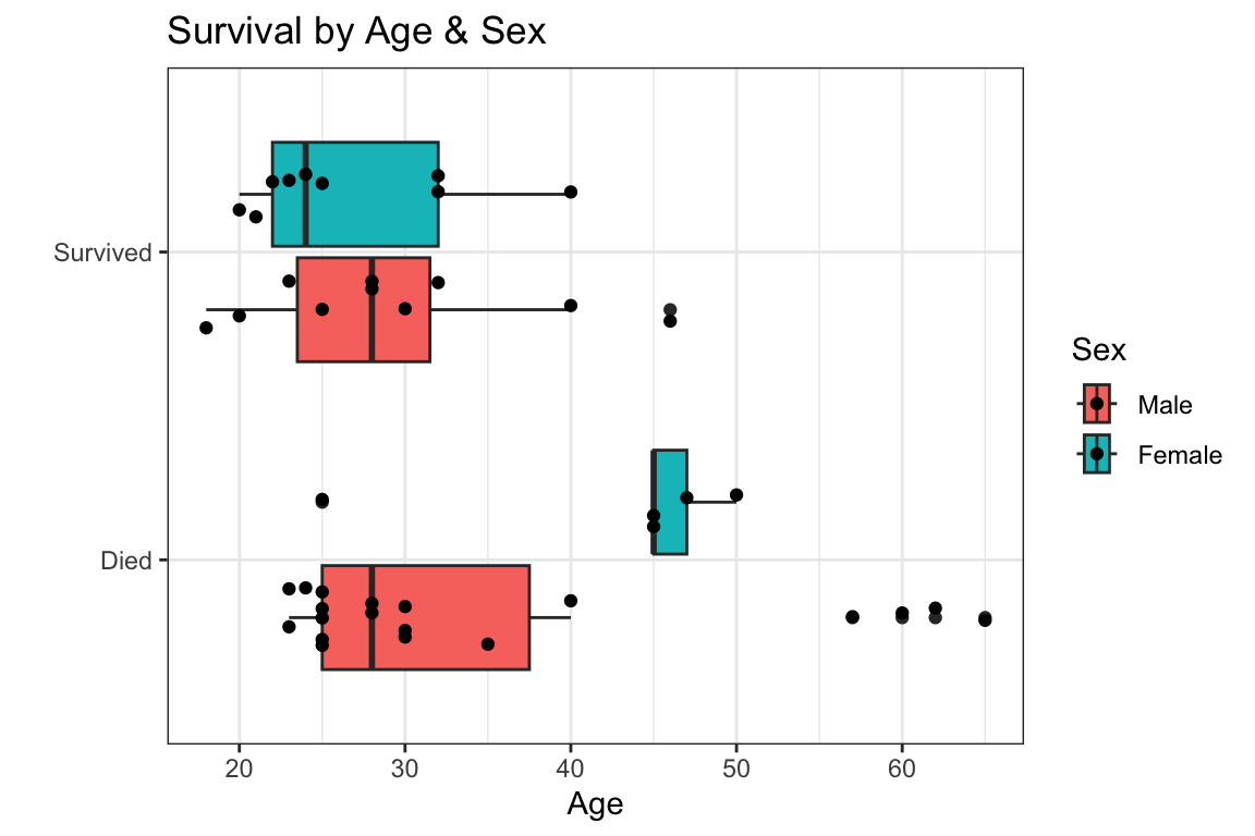
The Donner Party
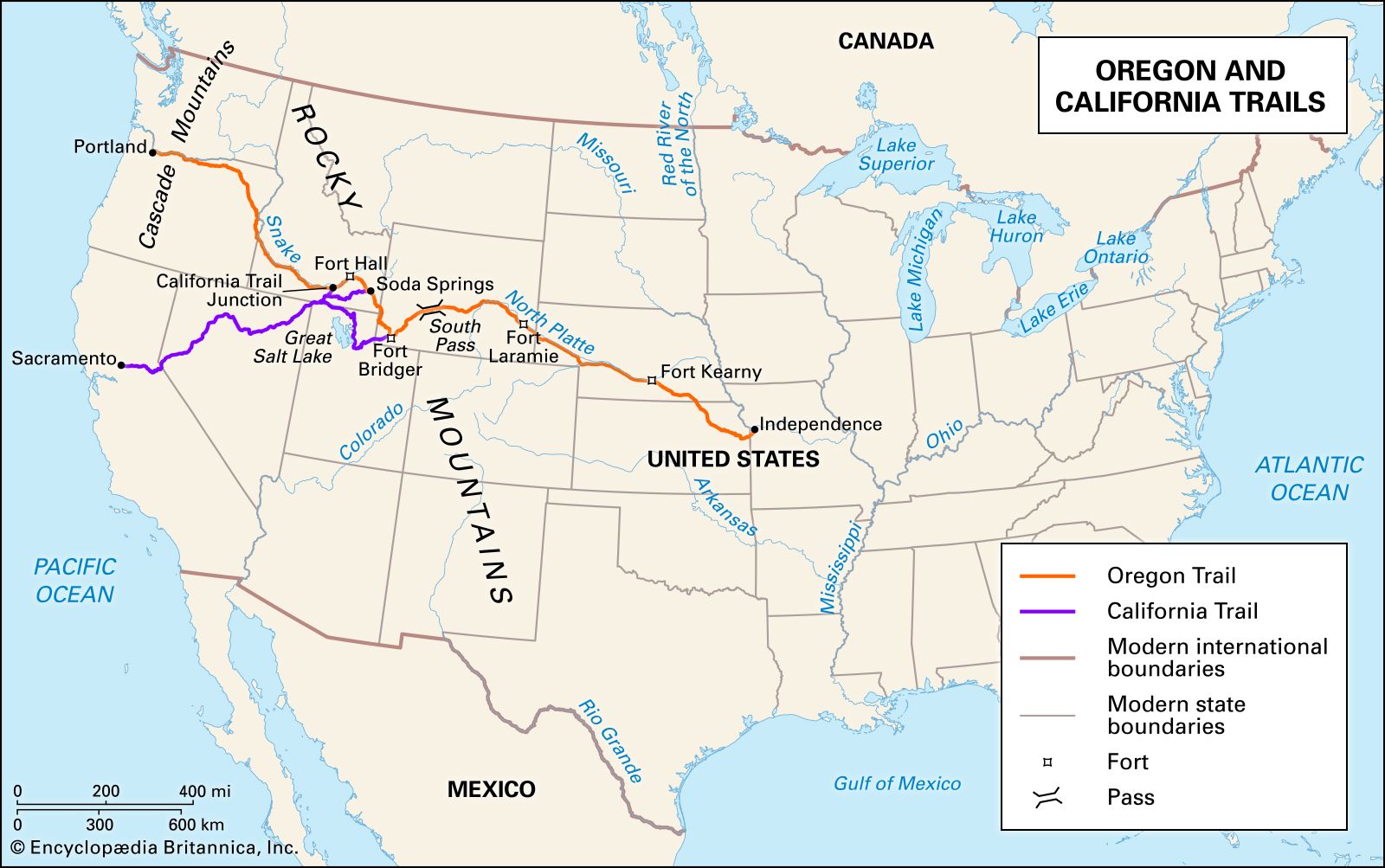
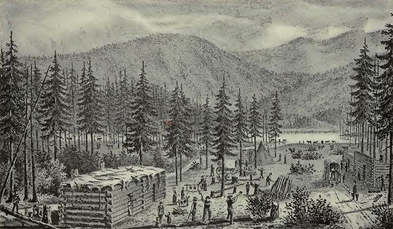
In 1846 the Donner and Reed families left Springfield, Illinois, for California by covered wagon. In July, the Donner Party, as it became known, reached Fort Bridger, Wyoming. There its leaders decided to attempt a new and untested rote to the Sacramento Valley. Having reached its full size of 89 people and 20 wagons, the party was delayed by a difficult crossing of the Wasatch Range and again in the crossing of the desert west of the Great Salt Lake. The group became stranded in the eastern Sierra Nevada mountains when the region was hit by heavy snows in late October. By the time the last survivor was rescued on April 21, 1847, 41 of the 89 members had died from famine and exposure to extreme cold.
The Donner Party
The Donner Party
The Donner Party
The Donner Party
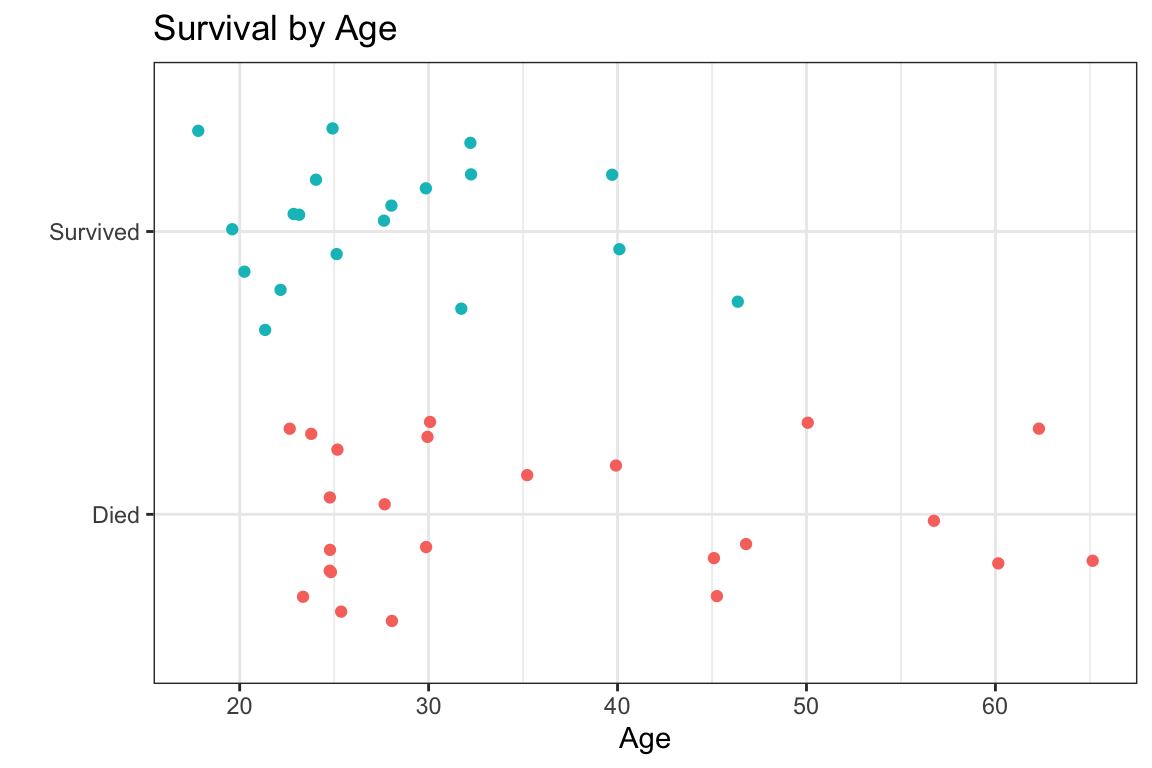
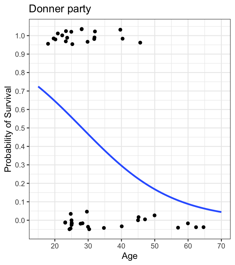
- what’s the probability of survival given age?
- logistic regression models the probability of a binary outcome as a function of one or more predictors
- e.g. probability of
Status(binary outcome:SurvivedvsDied) as a function ofAge(continuous variable)
The Donner Party
Code
donner %>%
    mutate(prob = ifelse(Status == "Survived", 1, 0)) %>%
    ggplot(aes(x=Age, y=prob, color=Sex)) +
       geom_jitter(height=0.025, width=0) +
       lims(x=c(15,70), y=c(-0.1,1.1)) +
       scale_y_continuous(breaks=seq(0,1,0.1)) +
       geom_smooth(method="glm", method.args=list(family="binomial"), se=FALSE, fullrange=TRUE) +
       labs(title="Donner party", y="Probability of Survival") +
       theme_bw()
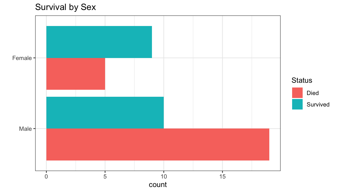
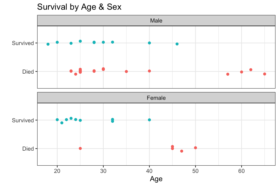
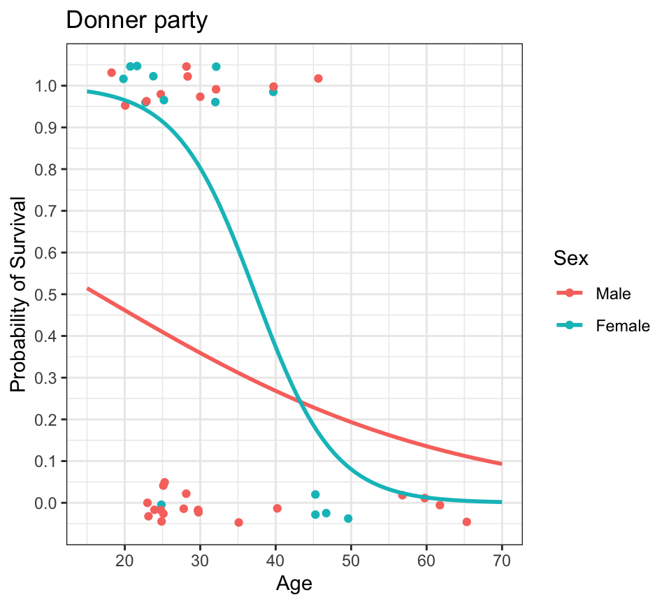
- what’s the probability of survival as a function of age, by sex?
- we can plot a logistic regression fit in
ggploteasily usinggeom_smooth() - logistic regression lines are usually S-shaped (sigmoidal)
Logistic Regression
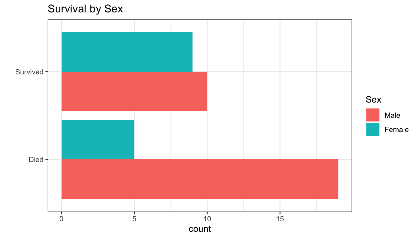
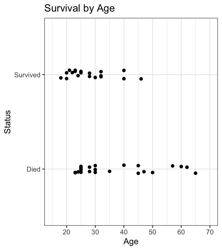
- these are all descriptive ways of looking at the relationship between characteristics (age, sex) and probability of survival
- logistic regression can give us a quantitative way of describing these relationships
Why not linear regression?
Code
donner %>%
    mutate(prob = ifelse(Status == "Survived", 1, 0)) %>%
    filter(Sex=="Female") %>%
    ggplot(aes(x=Age, y=prob)) +
       geom_jitter(height=0.05, width=0, color="black") +
       scale_y_continuous(breaks=seq(0,1,0.1)) +
       geom_smooth(method="lm", se=FALSE, fullrange=TRUE, color="orange") +
       lims(x=c(0,80), y=c(-0.5,1.5)) +
       labs(title="Donner party (Females)", y="Probability of Survival") +
       theme_bw()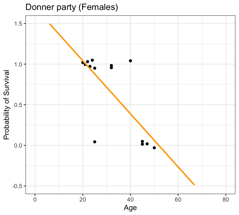
- linear regression model prediction extends above 1.0 and below 0.0
- doesn’t make any sense given the thing we’re trying to model is a probability
- probabilities can only live between 0.0 and 1.0
Why not linear regression?
Code
donner %>%
    mutate(prob = ifelse(Status == "Survived", 1, 0)) %>%
    filter(Sex=="Female") %>%
    ggplot(aes(x=Age, y=prob)) +
       geom_jitter(height=0.05, width=0) +
       scale_y_continuous(breaks=seq(0,1,0.1)) +
       geom_smooth(method="lm", se=FALSE, fullrange=TRUE, color="orange") +
       geom_smooth(method="glm", method.args=list(family="binomial"), se=FALSE, fullrange=TRUE, color="blue") +
       lims(x=c(5,70), y=c(-0.5,1.5)) +
       labs(title="Donner party (Females)", y="Probability of Survival") +
       theme_bw()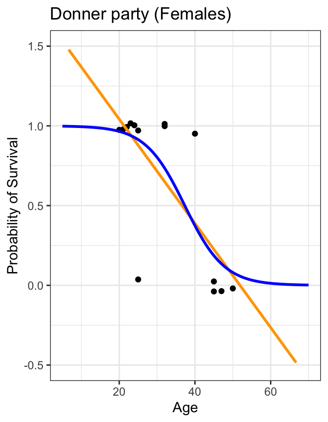
Also: we violate assumptions of linear regression
- linearity: relationship between predictor and outcome is not linear
- normality: residuals are not normally distributed
- homoscedasticity: variance of residuals is not constant over the range of the predictor variable
Logistic Regression
Code
donner %>%
    mutate(prob = ifelse(Status == "Survived", 1, 0)) %>%
    filter(Sex=="Female") %>%
    ggplot(aes(x=Age, y=prob)) +
       geom_jitter(height=0.05, width=0) +
       scale_y_continuous(breaks=seq(0,1,0.1)) +
       geom_smooth(method="glm", method.args=list(family="binomial"), se=FALSE, fullrange=TRUE, color="blue") +
       lims(x=c(5,70), y=c(-0.05,1.05)) +
       labs(title="Donner party (Females)", y="Probability of Survival") +
       theme_bw()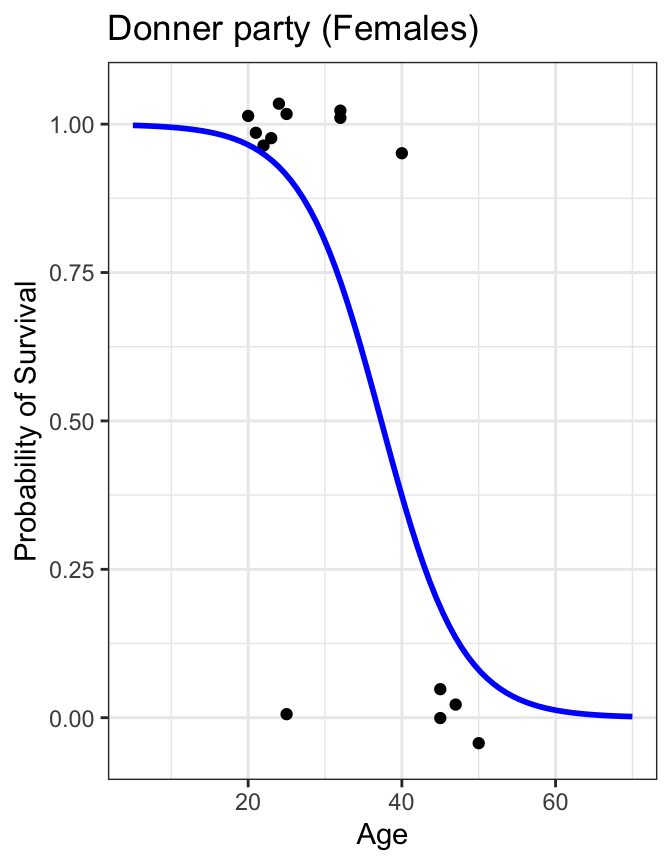
- we can treat Survived and Died as successes and failures arising from a binomial distribution where the probability of a success is given by a transformation of a linear model of the predictor(s)
- this is a general way of addressing this type of problem in regression, and the resulting models are called generalized linear models (GLMs)
- Logistic regression is just one example of a GLM
- but first: a reminder of the binomial distribution
Binomial Distribution
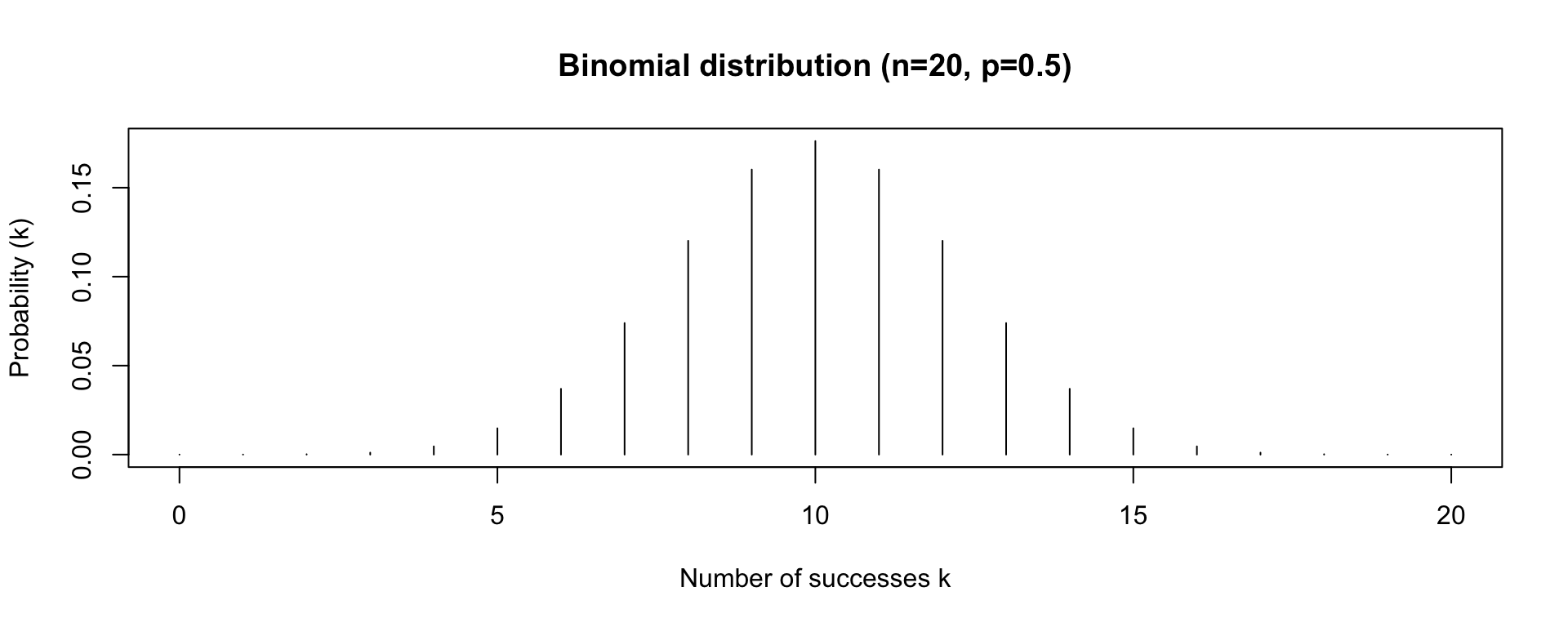
- the Binomial distribution has two parameters: n the number of trials, and p the probability of success on a given trial
- the Binomial distribution gives us the probability of observing k successes in n trials, given p
- e.g. probability of observing 3 heads in 20 coin flips, given that the probability of heads is 0.5
Binomial Distribution
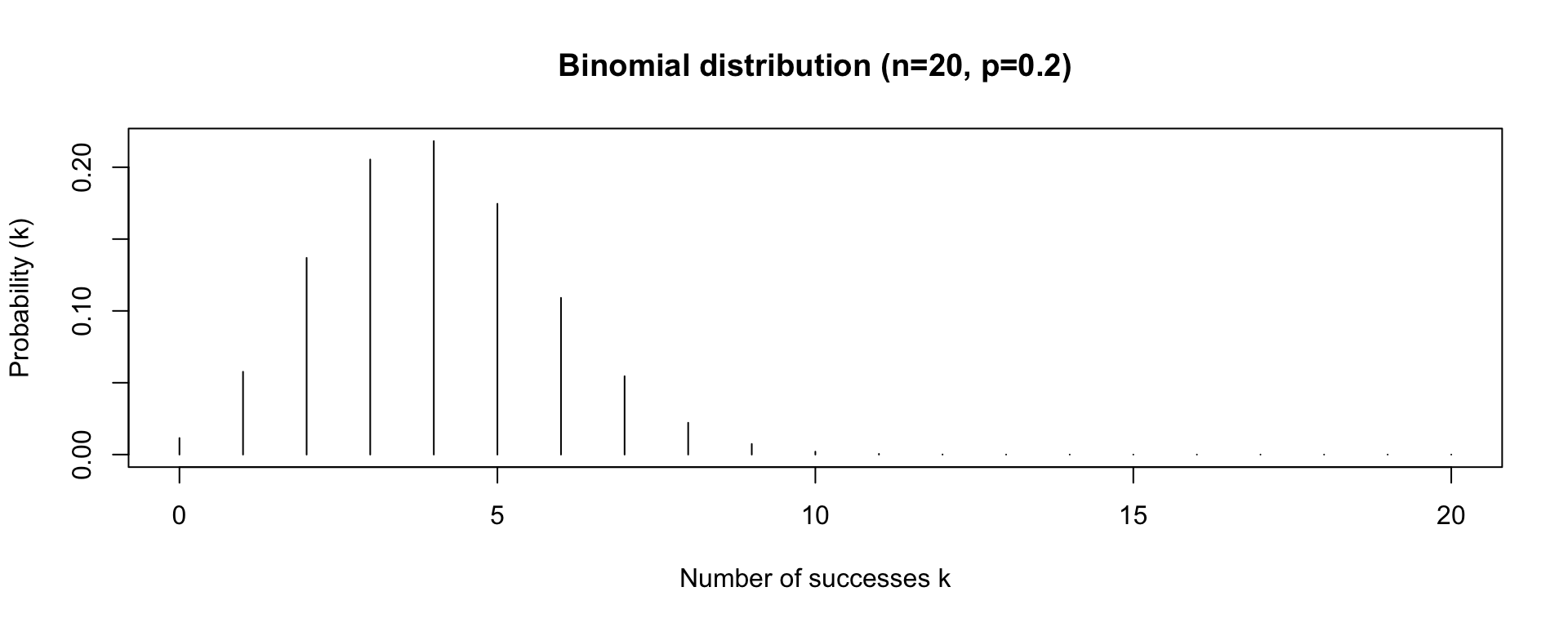
- the Binomial distribution has two parameters: n the number of trials, and p the probability of success on a given trial
- the Binomial distribution gives us the probability of observing k successes in n trials, given p
- e.g. probability of observing 3 heads in 20 coin flips, given that the probability of heads is 0.2
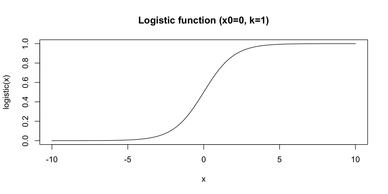
Properties of the Logit Function
- the Logit function is the inverse of the Logistic function
- the Logistic function is an S-shaped curve that maps continuous values (-\infty to \infty) to the interval (0,1)
Logistic Regression in R
Call:
glm(formula = Status ~ Age, family = binomial, data = donner)

Coefficients:
            Estimate Std. Error z value Pr(>|z|)
(Intercept)  2.06749    1.09914   1.881   0.0600 .
Age         -0.07339    0.03510  -2.091   0.0366 *
---
Signif. codes:  0 '***' 0.001 '**' 0.01 '*' 0.05 '.' 0.1 ' ' 1

(Dispersion parameter for binomial family taken to be 1)

    Null deviance: 59.028  on 42  degrees of freedom
Residual deviance: 53.134  on 41  degrees of freedom
AIC: 57.134

Number of Fisher Scoring iterations: 4- the model is: log\left(\frac{p}{1-p}\right) = 2.07 - 0.07(\mathrm{Age})
- or, equivalently: p = \frac{e^{2.07 - 0.07(\mathrm{Age})}}{1 + e^{2.07 - 0.07(\mathrm{Age})}}
Code
donner %>%
mutate(prob = ifelse(Status == "Survived", 1, 0)) %>%
ggplot(aes(x=Age, y=prob)) +
geom_jitter(height=0.05, width=0) +
scale_y_continuous(breaks=seq(0,1,0.1)) +
geom_smooth(method="glm", method.args=list(family="binomial"), se=FALSE, fullrange=TRUE, color="blue") +
lims(x=c(5,70), y=c(-0.05,1.05)) +
labs(title="Donner party (Males & Females)", y="Probability of Survival") +
theme_bw()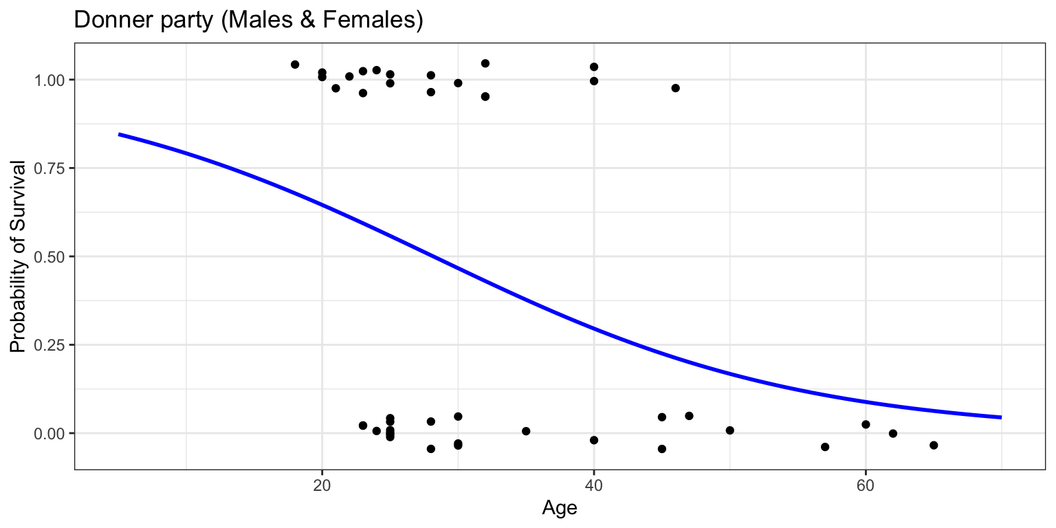
Prediction with Logistic Regression
Call:
glm(formula = Status ~ Age, family = binomial, data = donner)

Coefficients:
            Estimate Std. Error z value Pr(>|z|)
(Intercept)  2.06749    1.09914   1.881   0.0600 .
Age         -0.07339    0.03510  -2.091   0.0366 *
---
Signif. codes:  0 '***' 0.001 '**' 0.01 '*' 0.05 '.' 0.1 ' ' 1

(Dispersion parameter for binomial family taken to be 1)

    Null deviance: 59.028  on 42  degrees of freedom
Residual deviance: 53.134  on 41  degrees of freedom
AIC: 57.134

Number of Fisher Scoring iterations: 4- what is the probability of survival for a 40-year-old?
        1
0.2956287
Code
donner %>%
    mutate(prob = ifelse(Status == "Survived", 1, 0)) %>%
    ggplot(aes(x=Age, y=prob)) +
       geom_jitter(height=0.05, width=0) +
       scale_y_continuous(breaks=seq(0,1,0.1)) +
       geom_smooth(method="glm", method.args=list(family="binomial"), se=FALSE, fullrange=TRUE, color="blue") +
       lims(x=c(5,70), y=c(-0.05,1.05)) +
       geom_vline(xintercept=40, color="red") +
       geom_hline(yintercept=prob_40, color="red") +
       labs(title="Donner party (Males & Females)", y="Probability of Survival") +
       theme_bw()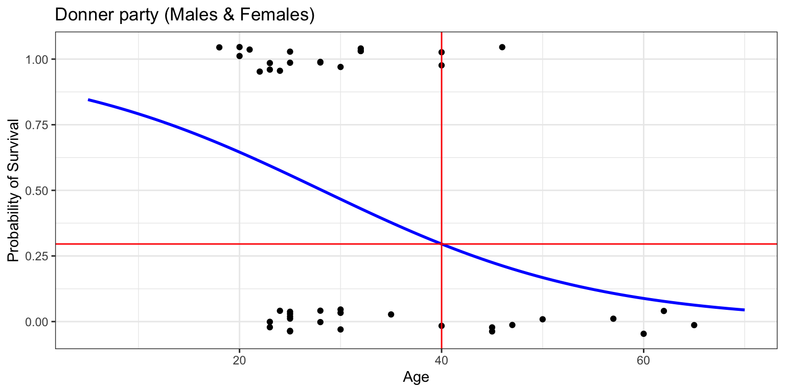
Logistic Regression with 2 Predictors
(Intercept)         Age   SexFemale
 2.00466996 -0.08762745  1.50667376
Code
donner %>%
    mutate(prob = ifelse(Status == "Survived", 1, 0)) %>%
    ggplot(aes(x=Age, y=prob, color=Sex)) +
       geom_jitter(height=0.05, width=0) +
       scale_y_continuous(breaks=seq(0,1,0.1)) +
       geom_smooth(method="glm", method.args=list(family="binomial"), se=FALSE, fullrange=TRUE) +
       lims(x=c(5,70), y=c(-0.05,1.05)) +
       labs(title="Donner party", y="Probability of Survival") +
       theme_bw()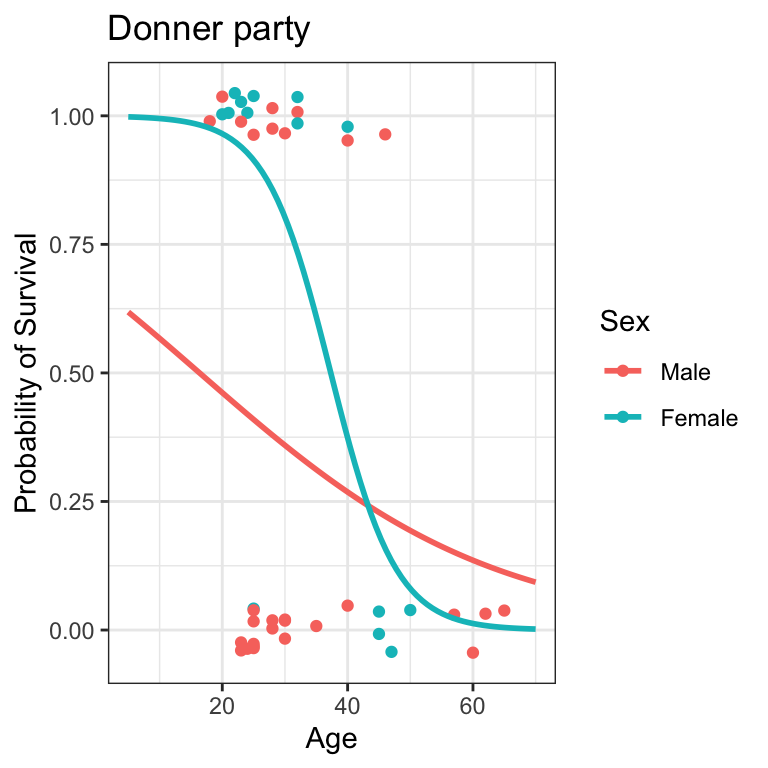
\begin{matrix} log\left(\frac{p}{1-p}\right) &= &2.0 - 0.09(\mathrm{Age}) + 1.5(\mathrm{SexFemale})\\ p &= &\frac{e^{2.0 - 0.09(\mathrm{Age}) + 1.5(\mathrm{SexFemale})}}{1 + e^{2.0 - 0.09(\mathrm{Age}) + 1.5(\mathrm{SexFemale})}} \end{matrix}
Check for log-odds linearity
- are the predictors linearly related to the log odds of the outcome?
cut()the predictorAgeinto bins usingquantile()- within each bin, compute log odds of
Survived
Code
donner %>%
    mutate(prob = ifelse(Status == "Survived", 1, 0)) %>%
    ggplot(aes(x=Age, y=prob)) +
       geom_jitter(height=0.05, width=0) +
       scale_y_continuous(breaks=seq(0,1,0.1)) +
       geom_smooth(method="glm", method.args=list(family="binomial"), se=FALSE, fullrange=TRUE, color="blue") +
       geom_vline(xintercept=quantile(donner$Age), color="red", lty=2) +
       lims(x=c(5,70), y=c(-0.05,1.05)) +
       labs(title="Donner party", y="Probability of Survival") +
       theme_bw()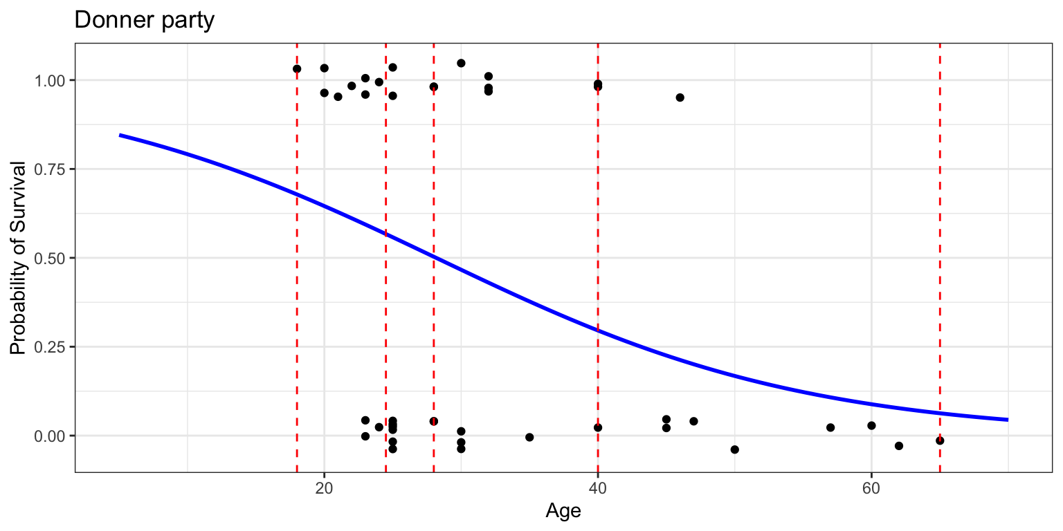
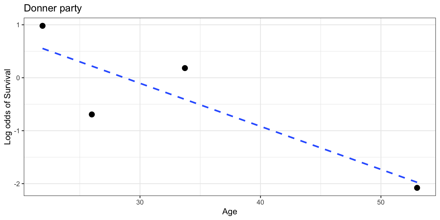
Check for log-odds linearity
- then plot age vs log odds of survival within each quantile bin
- is it linear? sort of. maybe not.
- (second bin should be higher)
- but we don’t have much data in this toy dataset so 🤷
- you will see an example in the homework this week of a larger dataset
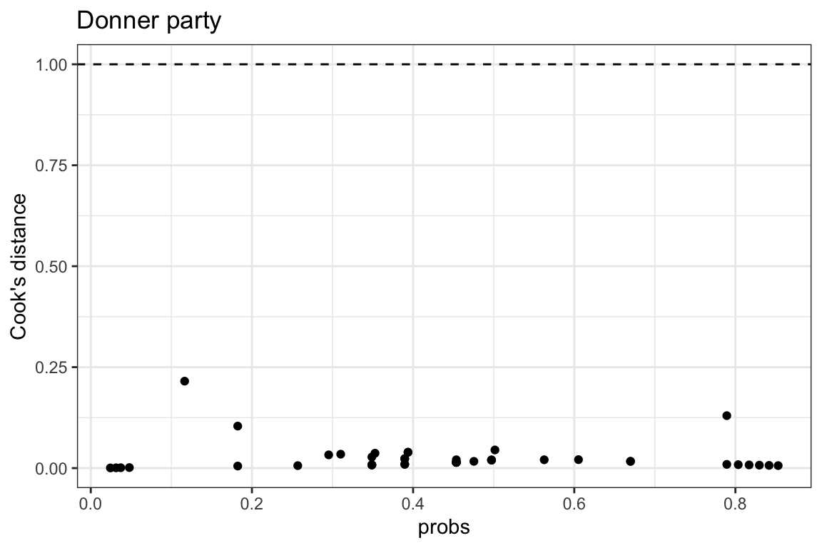
Outliers
- use Cook’s distance
- Cook’s distance is a measure of the influence of each observation on the model
- observations with high Cook’s distance are outliers
- values > 1 are considered high
- all our values are < 1 so we’re ok