library(tidyverse)
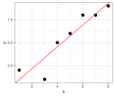
x <- c(1,4,3,6,5,7,8)
y <- c(2,5,1,8,6,8,9)
n = 7
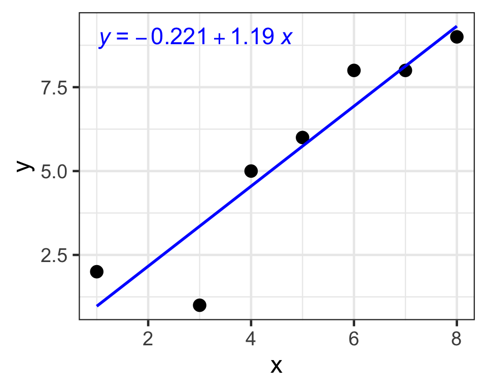
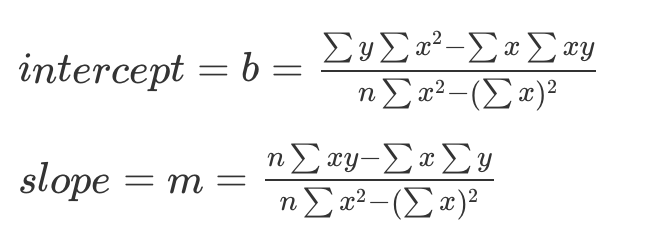
(b <- ((sum(y)*sum(x^2)) - (sum(x)*sum(x*y))) / ((n*sum(x^2)) - (sum(x))^2))[1] -0.2213115[1] 1.192623Week 3
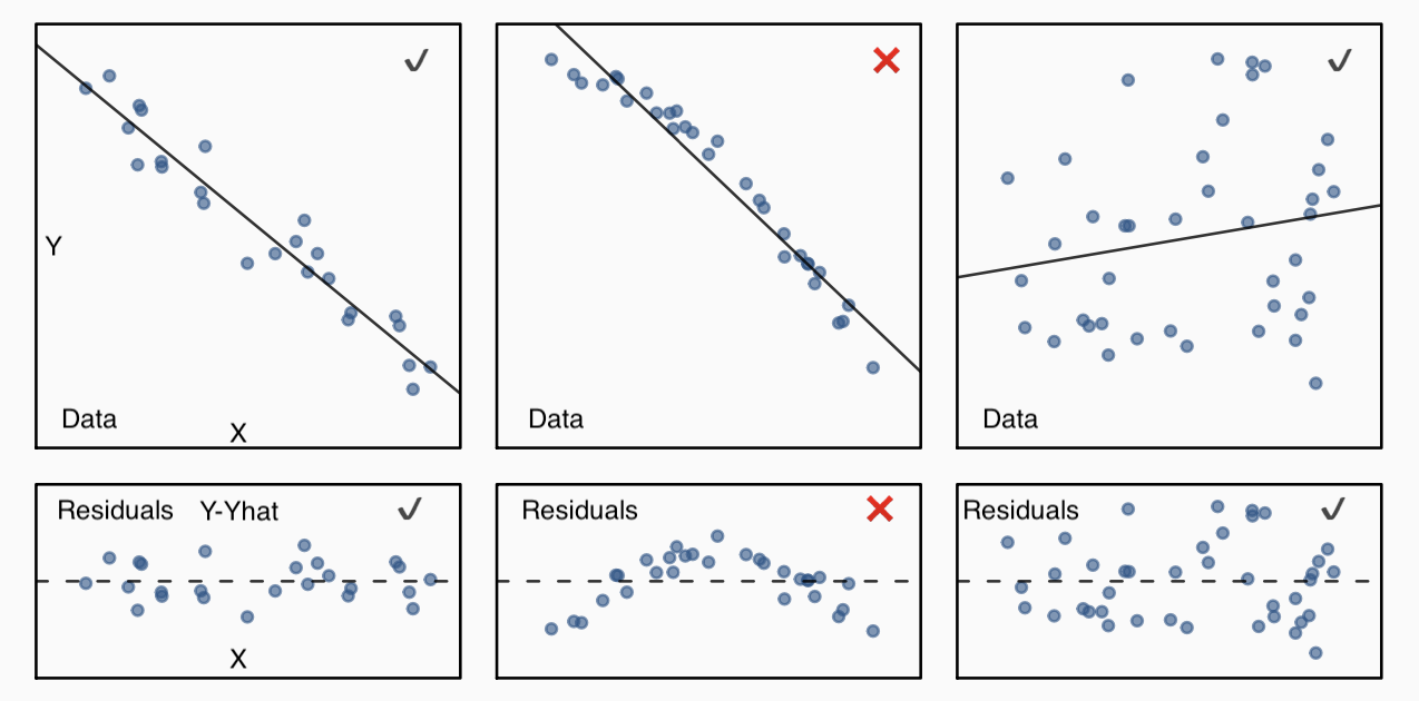
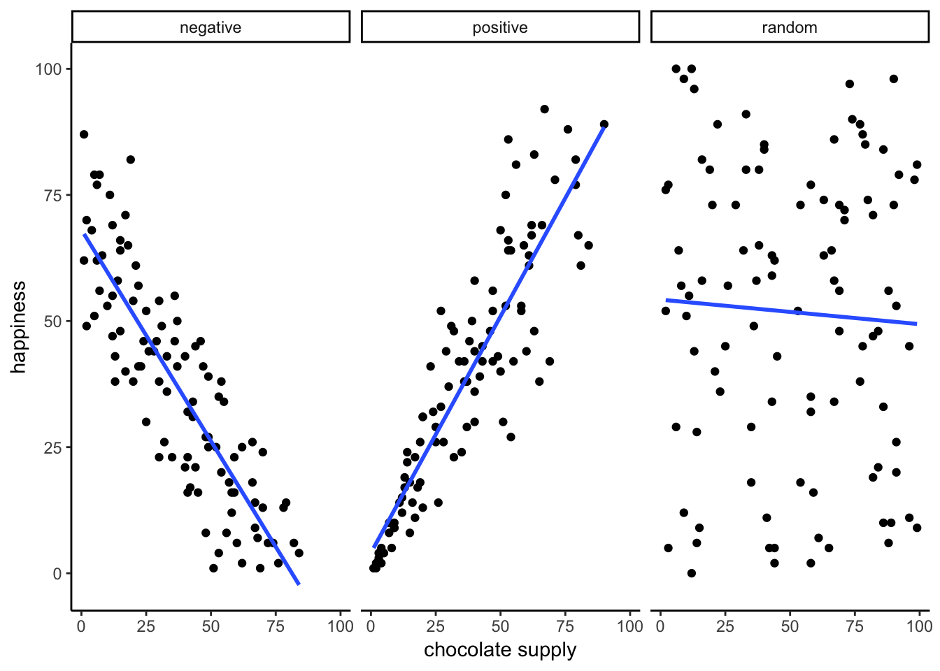
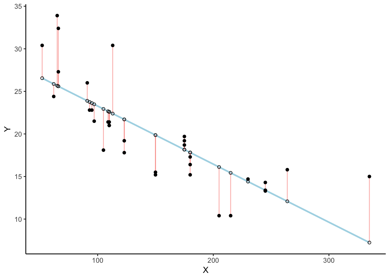
regression minimizes the sum of the (squared) residuals
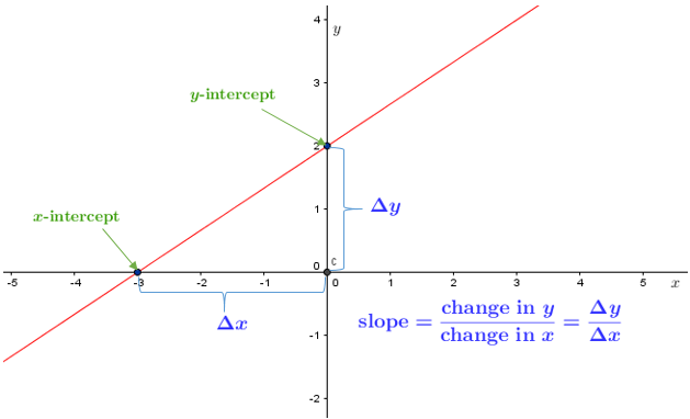
y = mx +b
y = \text{slope}*x + \text{yintercept}
We will also use this form:
y = \beta_{0} + \beta_{1}x
Y = mX + b


b = -0.221
m = 1.19
Y = (1.19)X - 0.221
lm()What does the y-intercept mean?
It is the value where the line crosses the y-axis when x = 0
What does the slope mean?
The slope tells you the rate of change.
For every 1 unit of X, Y changes by “slope” amount
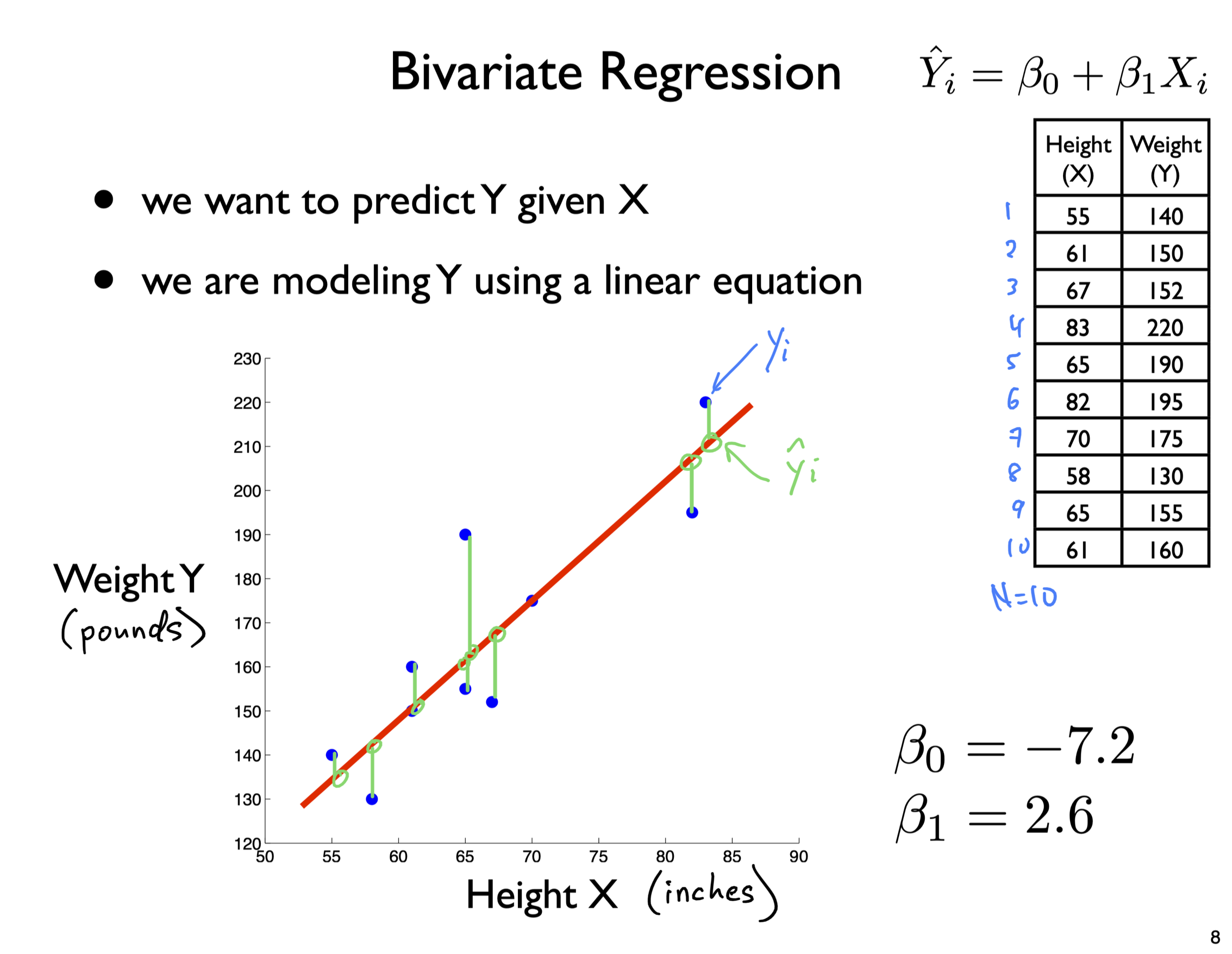
E.g., slope = 2.6
then for every 1 unit of X
Y increases by 2.6 units
Y_{i} = \hat{Y_{i}} + \varepsilon_{i}
\hat{Y}_{i} = \beta_{0} + \beta_{1} X_{i}
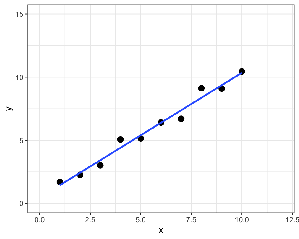
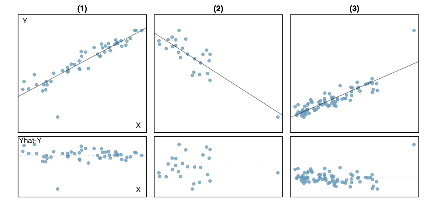
sum of squared residuals = 1.9sum of squared total = 82.6R-squared = 0.98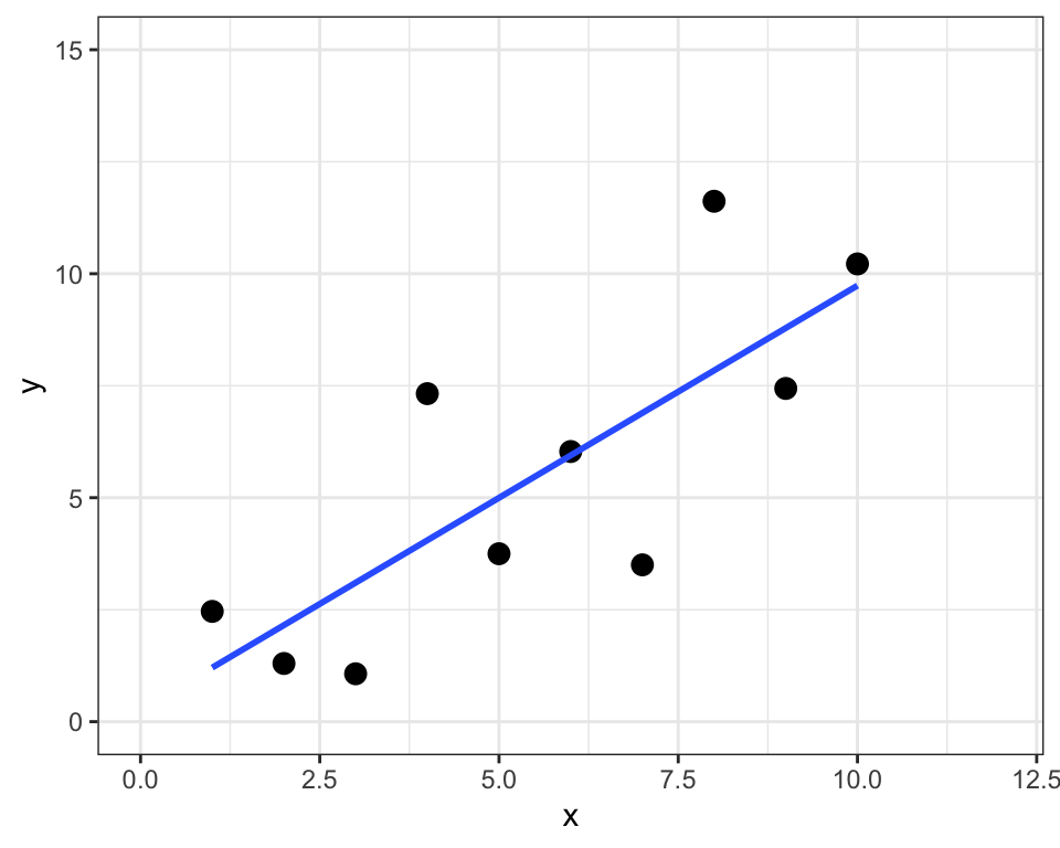
sum of squared residuals = 46.5sum of squared total = 120.6R-squared = 0.61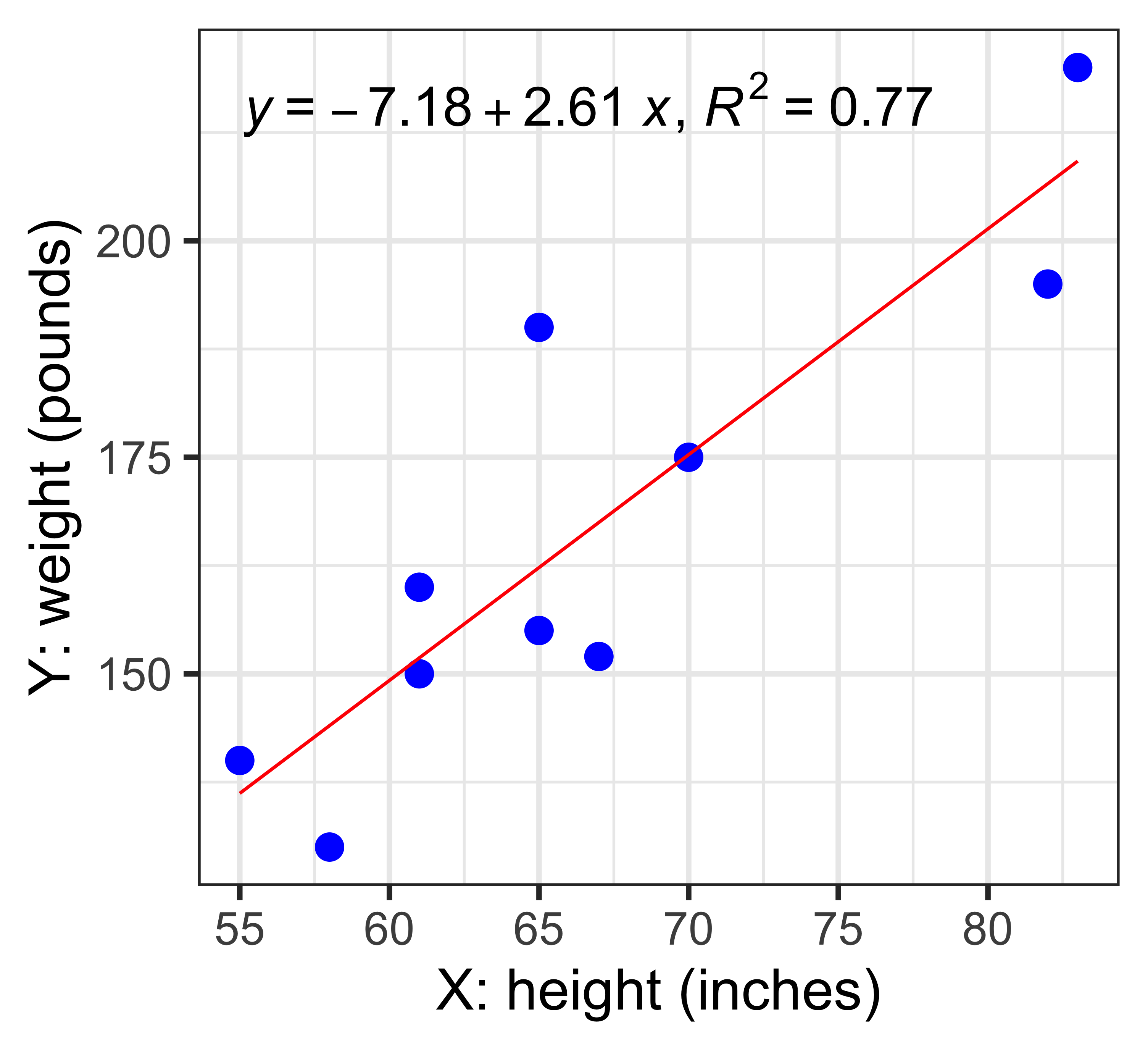
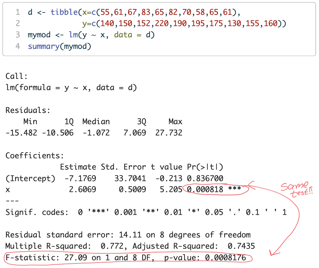
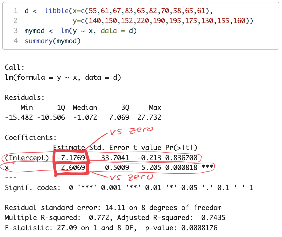
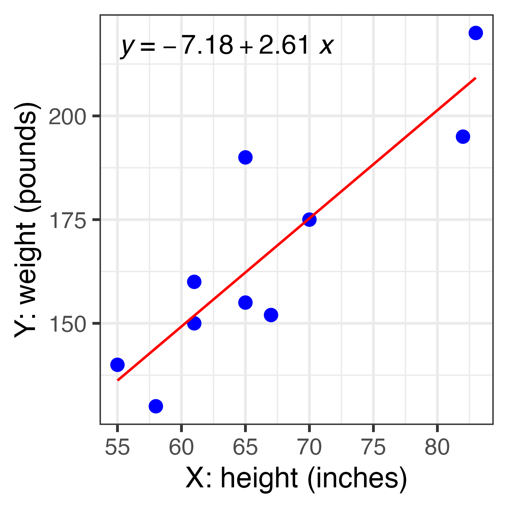
Y = -7.2 + 2.6 X
R^{2} = 0.772
s_{est} = 14.11 (pounds)
summary() of our lm() in R: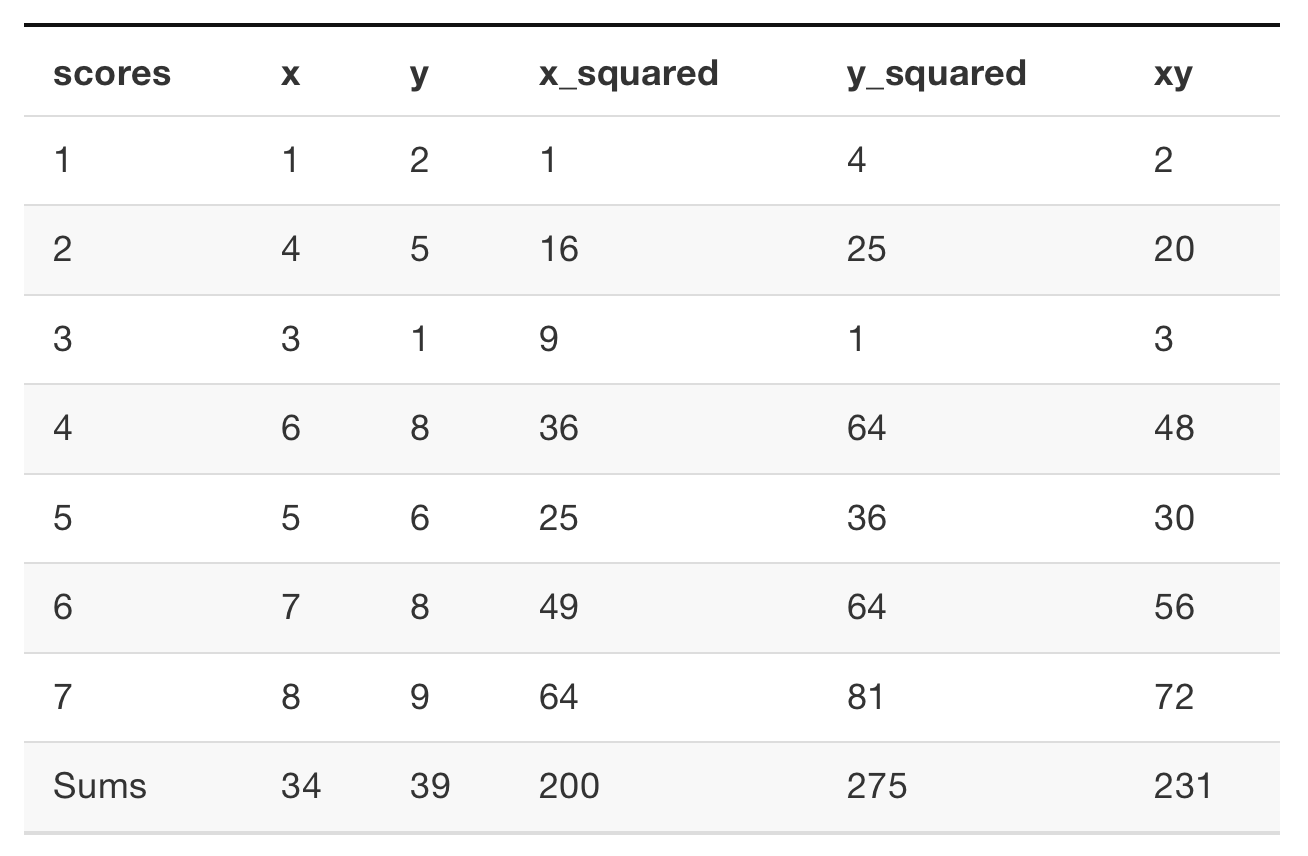
summary() of our lm() in R: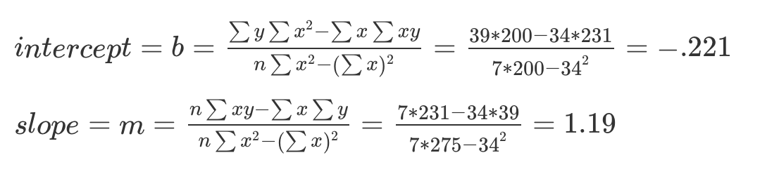
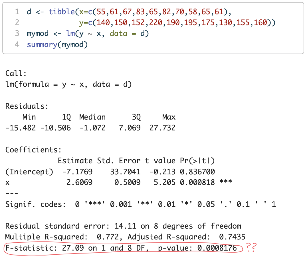
F(1,8)=27.09
p=0.0008176
→ what is this hypothesis test of?